---

In the last post we had started a case study example for regression analysis to help an investment firm make money through property price arbitrage (read part 1 : regression case study example). This is an interactive case study example and required your help to move forward. These are some of your observations from exploratory analysis that you shared in the comments of the last part (download the data here)

Katya Chomakova : The house prices are approximately normally distributed. All values except the three outliers lie between 1492000 and 10515000. Among all numeric variables, house prices are most highly correlated with Carpet (0.9) and Builtup(0.75).
Mani : Initially, it appears as if housing price has good correlation with built up and carpet. But, once we remove all observations having missing values (which is just ~4% of total obs), I find that the correlation drops down very low (~0.09 range)

Katya and Mani noticed something unusual about missing observations and outliers in the data, and how their presence and absence were changing the results dramatically. This is the reason data preparation is an important exercise for any machine learning or statistical analysis to get consistent results. We will learn about data preparation for regression analysis in this part of the case study. Before we explore this in detail, let’s take a slight detour to understand the crux of stability and talk about fall of heroes.

Every kid needs a hero. I had many when I was growing up. This is a story of how I used a concept in physics caller ‘center of gravity‘ to chose one of my heroes by having an imaginary competition between:

Mike Tyson Vs. Bop Bag

The Champion : Mike Tyson was the undisputed heavyweight boxing champion in the late 1980s. He was no Mohammad Ali but was on his path to come closest to The Greatest. This is where things went wrong for Tyson; he was convicted of rape and was in prison for 3 years. Out of jail and desperate to regain his glory days, Tyson challenged Evander Holyfield,the then undisputed champion. What followed was a disgrace for any sport where during the challenge match Tyson bit a part of Holyfield’s ear off and got disqualified.

The Challenger : Most of us have played with a bop bag or the punching toy as kids. It is designed in such a way that when punched, it topples for a while but eventually stands back up on its own. Bop bag is a perfect example where the center of gravity of the object is highly grounded and stays within its body. You could punch it, kick it, or perturb it in any possible way but the bop bag will stand back up after a fall – yes, it has that cute, funny smile too. On the other hand, like Mike Tyson, most of us struggle big time after a fall. Possibly because our center of gravity is outside our body in other people’s opinion about us. Tyson was mostly driven by the praises from others after a win rather than his love for the game.

The Winner : Center of gravity helped me choose my hero : bop bag. This cute toy reminds me every day to keep my center grounded and inside my body and not let others perturb my core – even when punched. I wish I could always wear a sincere smile like my hero.

Bop bag also has important lessons for data preparation for machine learning and data science models. The data for modeling needs to display stability similar to bop bag and must not give completely different results with different observations. Katya and Mani have noticed a major instability in our data in their exploratory analysis. They have highlighted the presence of missing data and outliers; we will explore these ideas further in this part when we will explore data preparation for regression analysis. Now, let’s go back to our case study example.

Data Preparation for Regression – Case Study Example

You are a data science consultant for an investment firm that tries to make money through property price arbitrage. They get daily data for thousands of houses across the country available for sale. Their expectation from you is to suggest properties worth investing in. This requires you to identify properties selling at a lower price than the market price. You already have quoted prices for all the properties. Now, you need to create a model to estimate market price for properties. Your client should invest in the properties with a higher estimated price than the quoted price.

In your effort to create a price estimation model, you have gathered this data. The next step is data preparation for regression analysis before the development of a model. This will require us to prepare a robust and logically correct data for analysis.

We will do our analysis for this case study example on R. For this I recommend you install R & R Studio on your system. However, you could also try these codes on this online R engine : R-Fiddle.

We will first import the data in R and then prepare a summary report for all the variables using this command:

data<-read.csv('http://ucanalytics.com/blogs/wp-content/uploads/2016/07/Regression-Analysis-Data.csv')

summary(data)

A version of the summary report is displayed here. Remember there are total 932 observations is this data set.

	Dist_Taxi	Dist_Market	Dist_Hospital	Carpet	Builtup
Min.	146	1666	3227	775	932
1st Qu.	6476	9354	11302	1318	1583
Median	8230	11161	13163	1480	1774
Mean	8230	11019	13072	1512	1795
3rd Qu.	9937	12670	14817	1655	1982
Max.	20662	20945	23294	24300	12730
NA’s	13	13	1	8	15

Look at the last row where all the above variables have some missing data. Parking and City_Category are categorical variables hence we have got levels for them. Notice there is missing data in Parking as well marked as ‘Not Provided’.

Parking	City_Category		Rainfall	House_Price
Covered : 188 No Parking: 145 Not Provided : 227 Open : 372	CAT A: 329 CAT B: 365 CAT C: 238	Min.	110	30000
		1st Qu.	600	4658000
		Median	780	5866000
		Mean	785.6	6084695
		3 Qu.	970	7187250
		Max.	1560	150000000
		NA’s	0	0

The first thing we will do is to remove missing variables from this dataset. We will explore later whether removal of missing variables is a good strategy or not. We will also calculate how many observations we will lose by removing missing data.

data_without_missing<-data[complete.cases(data),]

nrow(data) - nrow(data_without_missing)

We have lost 34 observations after removal of missing data. The data set is now down to 898 observations. This is ~4% observations as Mani pointed in his comment. Also, notice that missing variables for categorical variables (Parking) are not removed, could you reason why?

In the next step, we will plot a box plot of housing price to identify outliers for the dependent variable.

options(scipen = 100) # this will print the numbers without scientific notation

boxplot(data_without_missing$House_Price, col = "Orange",main="Box Plot of House Price")

 

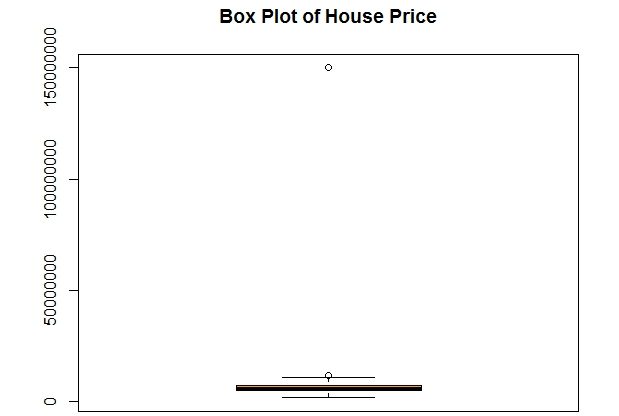Clearly, there is an extreme outlier in this dataset. The dot at the top represents that outlier. All the other data-points are packed in the almost flat box at the bottom. (Click on the image to enlarge it)

Let’s try to look at this extreme outlier by fetching this observation.

data_without_missing[data_without_missing$House_Price>10^8,]

This observation seems to be for a large mansion in some countryside. As can be seen in data when compared with the summary data for other observations.

Dist_Taxi	Dist_Market	Dist_Hospital	Carpet	Builtup	Parking	City_Category	Rainfall	House_Price
20662	20945	23294	24300	12730	Covered	CAT B	1130	150000000

There is no point in keeping this super-rich property in data while preparing a model for middle-class housing. Hence we will remove this observation. The next step is to look at the box plot of all the numerical variables in the model to find unusual observations. We will normalize the data to bring it to the same scale.

boxplot(scale(data_without_missing[data_without_missing$House_Price<10^8,c(2:6,9:10)]),col="Orange")

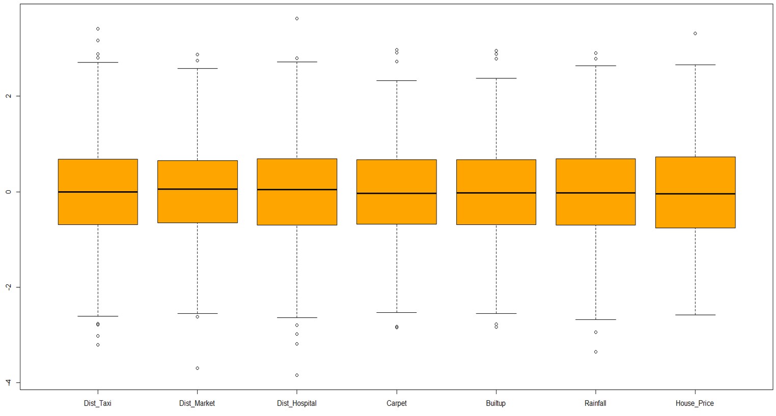This data looks fairly centered as is required for most modeling techniques.

Sign-off Note

In this part, we have primarily spent our time on univariate analysis for data preparation for regression. In the next part, we will explore patterns through bivariate analysis before the development of multivariate models. These are some of the questions you may want to ponder and share your view before the next part:

1) We had removed 34 observations with missing data, what impact the removal of missing data can have on our analysis? Could we do something to minimize this impact?

2) Why did we not remove missing values from the categorical variable i.e. Parking?

3) What impact could the extreme outlier, a large mansion, have on the model we are developing for middle-class house prices? Was it a good idea to remove that outlier?