
Death and Principal Component Analysis – by Roopam
Principal component analysis is a wonderful technique for data reduction without losing critical information. Yes, you could reduce the size of 2GB data to a few MBs without losing a lot of information. This is like a mp3 version of music. Many, including some experienced data scientists, find principal component analysis (PCA) difficult to understand. However, I believe that after reading this article you will understand PCA and appreciate that it is a highly intuitive and powerful data science technique with several business applications. This article is a continuing part of our regression case study example where you are helping an investment firm make money through price arbitrage. In this article, I will help you gain the intuitive understanding of principal component analysis by highlighting both practical applications and the underlying mathematical fundamentals. Principal component analysis is also extremely useful while dealing with multicollinearity in regression models. In the subsequent article, we will use this property of PCA for the development of a model to estimate property price.
Before we explore further nuances of principal component analysis, in the true tradition of YOU CANalytics, let’s digress a bit and create links between:
Principal Component Analysis and Death
 What happens when people die? Where do they go? All of us have pondered this at some point or other. There are several religious and a few non-religious theories to explain events after death. A theory which makes sense to me is: after death, we go back to our fundamental elements. Here, I am not talking about metaphysical or divine elements but chemistry. There are close to 120 known elements including lithium, oxygen, uranium, hydrogen, argon, and carbon. These elements form the periodic table we learned in the chemistry lessons in high-school. Despite the choice of roughly 120 elements, the human body does not have all of them in the same proportion. Incidentally, six elements, as shown in the chart, constitute close to 99% of the human body. Think of these elements as the principal components of the human body. The remaining ~1% of the human body has a little over 20 other elements. This means, around three-fourth of the elements in the periodic table are completely absent in the human body.
We noticed that about 1% of the human body has formed with ~ 20 elements. The idea with PCA is that if you remove these 20 elements you will lose just 1% of the essence of the human body. This will also mean that your information load will decline by ~77% (20/26). These ideas will form the basis of our understanding of principal component analysis as we progress with our pricing case study example. You could find the previous parts at this link: regression case study example.
Principal Component Analysis – Case Study Example
You had got a stern message from your client last evening. They want you to turn around the price estimation model soon so that they can integrate it into their business operations. Luckily, you have made a good progress while preparing your data for the regression modeling. The original data had some outliers and missing observations which you have decided to drop for this analysis. You can download the cleaned data from this link: regression-clean-data. In this analysis, you are trying to estimate the response variable (house price) through the other numeric and categoric predictor variables. This estimation will be used by your client, a property investment firm, to make money through price arbitrage.
In the previous part using bivariate analysis, we noticed that there is a significantly high correlation between some of the numeric predictor variables. This, you know, will create a problem of multicollinearity while regression model development. One of the most effective methods for elimination of multicollinearity is principal component analysis. I suggest you go back and read that article to get a good understanding of results of PCA (bivariate analysis). You have six numeric predictor variables in your dataset i.e.
|
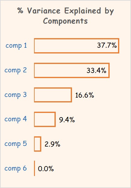 Before we jump to PCA, think of these 6 variables collectively as the human body and the components generated from PCA as elements (oxygen, hydrogen, carbon etc.). When you did the principal component analysis of these 6 variables you noticed that just 3 components can explain ~90% of these variables i.e. (37.7 + 33.4 + 16.6 = 87.7%). This means that you could reduce these 6 variables to 3 principal components by losing just 10% of the information. That is not a bad bargain 50% reduction in variables at the cost of 10% information. Moreover, these components will never have any multicollinearity between them as they are orthogonal or perfectly uncorrelated.
Later in this article, we will come back to how we have derived these components from our dataset. For now, let’s decipher the inner workings of principal component analysis. We will explore more about orthogonal components and variable reduction.
Let’s create a loose parallel to understand orthogonal rotation and loss of information which is at the core of PCA. A word of caution, this example is not how principal component analysis works but it will help you appreciate the inner workings of PCA. When you rotate your cell phone orthogonally (this is a fancy way of saying make it perpendicular) you kind of reduce the size of a landscape picture. Essentially, you are losing some information. Remember in the tilted states (i.e. positions between orthogonal states of the phone) the picture doesn’t change, hence we and PCA are not interested in non-orthogonal positions of the phone. PCA will find all the orthogonal positions for you with the quantum of information each position captures. Eventually, you will pick the positions of the phone that provide you with maximum information.
 For other kinds of pictures, i.e. a profile picture, the upright position is better than the horizontal position for the phone. Treat the pictures as data and principal component analysis is trying to find orthogonal positions (distinct components) for the phone to capture maximum information. Unlike the 2-dimensional world of the phone rotation, PCA rotates the axis in the n-dimensional world of the data. Here, n is equal to the number of variables. For our data with 6 variables, we have 6 orthogonal axes possible.
Now, you are ready to test these concepts and the mathematical theory behind them using the predictor variables in our dataset. The first thing we will do is extract principal components using R. Then we will also notice how Eigenvalues and Eigenvectors (yes those dreaded concepts we learned in matrix algebra in high school) are used to find the level of information and orthogonal axes.
To begin, let us prepare our data for PCA: (you can find the complete code on this link: principal-component-analysis-r-code)
data = read.csv('http://ucanalytics.com/blogs/wp-content/uploads/2016/09/Regression-Clean-Data.csv')
Now, tag the numeric predictor variables in the dataset for the principal component analysis.
numeric_predictors=c('Dist_Taxi','Dist_Market','Dist_Hospital','Carpet','Builtup','Rainfall')
Data_for_PCA = data[,numeric_predictors]
Now, that the data is ready for analysis. Let’s load a package called FactoMineR in R to run the principal component analysis.
if (!require('FactoMineR')) install.packages('FactoMineR')
pca=PCA(Data_for_PCA)
This command will generate a graph similar to this.

Here, distance to taxi, market, and hospital have formed a composite variable (comp 1) which explains 37.7% information in data. Another, orthogonal axis (comp 2) explains the remaining 33.4% of variation through the composite of carpet and built-up area. Rainfall is not a part of comp 1 or comp 2 but is a 3rd orthogonal component. You can get this information in a much more friendly tabular form to display composition of all the variables. Use this command in R.
pca$eig
| Components | Eigenvalue | % Variance Explained | Cumulative Variance (%) |
| comp 1 | 2.262 | 37.7% | 37.7% |
| comp 2 | 2.004 | 33.4% | 71.1% |
| comp 3 | 0.996 | 16.6% | 87.7% |
| comp 4 | 0.564 | 9.4% | 97.1% |
| comp 5 | 0.174 | 2.9% | 100.0% |
| comp 6 | 0.001 | 0.0% | 100.0% |
We have got the percentage of data (variance) explained by each component. Did you notice the second column named ‘Eigenvalue’? The eigenvalue is used in the principal component analysis to calculate the % variance explained. For instance, if you divide eigenvalue of comp 1 with the sum of all the eigenvalues {i.e. 2.262/(2.262+2.004…+0.001)} you will get 37.7%. Alright, so eigenvalue does have some cool properties.
Ok, what about eigenvectors? eigenvectors are the vector locations of these components. Matrix multiplication of our original dataset with ‘eigenvector-1’ will generate the dataset for comp 1. Similarly, you can generate data for other components as well. This has essentially, rotated our data for predictor variables on orthogonal (eigenvector) axes.
We can find the loading of our predictor variables on these components through a correlation matrix constructed with these commands in R.
Correlation_Matrix=as.data.frame(round(cor(Data_for_PCA,pca$ind$coord)^2*100,0))
Correlation_Matrix[with(Correlation_Matrix, order(-Correlation_Matrix[,1])),]
This correlation matrix tells us that 88% of the distance to the hospital is loaded on comp 1. 100% of both carpet and built-up area is loaded on comp 2.
| comp 1 | comp 2 | comp 3 | comp 4 | comp 5 | comp 6 | |
| Dist_Hospital | 88% | 0% | 0% | 2% | 10% | 0% |
| Dist_Taxi | 76% | 0% | 1% | 17% | 6% | 0% |
| Dist_Market | 61% | 0% | 0% | 38% | 1% | 0% |
| Rainfall | 1% | 1% | 98% | 0% | 0% | 0% |
| Carpet | 0% | 100% | 0% | 0% | 0% | 0% |
| Builtup | 0% | 100% | 0% | 0% | 0% | 0% |
If we remove component 4 to 6 from our data we will lose a little over 10% of the information. This also means that ~39% of the information available in ‘distance to market’ will be lost with component 4 & 5.
Now, you are feeling much more confident that you have addressed the issues of multicollinearity in the numeric predictor variables. You want to start with the development of regression models to estimate house prices.
Sign-off Note
In the human body after removing ~20 elements, we lost just 1% of the essence of the body. An important question, is this 1% responsible for something critical? You can’t ignore this question even while developing models with the principal components. Is it that the loss of 39% information captured in ‘distance to market’ will reduce the estimation power of our regression model? May be or may be not, we will see this when we will develop our first estimation model in the next post.
Excellent! Thank you
Very nice..
Hi Roopam, You articles have always been excellent. Keep the good work going. Also, I would be interested if you write an article on pricing optimization in analytics or suggest me any book or resource.
Thanks.
Try this book : Pricing and Revenue Optimization – by Robert Phillips.
Thanks you. Will look into it.
Is Part 5 coming up soon? It’s been a month and I’m starving for more of this case study!! 🙂
The last few weeks had been really hectic for me, that’s the reason for tardiness. Let me post the 5th part in a day or two. Cheers 🙂
Hello,
the below line of code
Correlation_Matrix[with(dd, order(-Correlation_Matrix[,1])),]
utilizes object dd,however dd has not been created by any prior code.
Thanks
Thanks for letting me know. Have corrected this typo.
Hello,
On using pca<-PCA(Data_for_PCA), there comes an error:
Error: could not find function "PCA"
What should I do?
Thanks.
You need to first install package FactoMineR in R. Use this command before using function PCA
if (!require(“FactoMineR”)) install.packages(“FactoMineR”)
Also, first you need to use:
library(‘FactoMineR’) after installing the package,if you are running as a standalone.
Thanks Roopam, Nice article, very informative!
I wanted to understand:(From the example above)
Does removing component 4 to 6 mean dropping variables: Rainfall, Carpet, Builtup from data-set?
No, that’s not correct. Here is one way to look: If you remove just component 6 (which has almost zero variance captured), you will not lose any information from the main variables. Additionally, removal of component 5 will also result in a negligible loss of information from the main variables. Collectively component 4-6 will result in loss of 10% information in the 6 main variables. This loss is predominantly for distance to market and taxi stand.
Thank You Roopam
When I am using these lines of code in my dataset
Correlation_Matrix=as.data.frame(round(cor(Data_for_PCA,pca$ind$coord)^2*100,0))
Correlation_Matrix[with(Correlation_Matrix, order(-Correlation_Matrix[,1])),]
I am getting the output of all the dimesions as NA
How to solve this issue?
Hi Roopam. Thank you. This is for the first time I have understood PCA!!
One question : Can we do PCA for categorical/qualitative variables? if no, then why not? And if PCA does not work for categorical variables then what is the alternative to handle dimensionality reduction for categorical variables?
Thanks, Dhara. Glad I could help you get an intuitive understanding of PCA.
PCA doesn’t work for categorical variables unless you convert the categorical variables to numeric through a transformation such as the weight of evidence (WoE). http://ucanalytics.com/blogs/information-value-and-weight-of-evidencebanking-case/
excellent
Thank for your work Roopam.
Please help me with this Error:
Error in data[, numeric_predictors] : object of type ‘closure’ is not subsettable
I don´t know what it means.
Excellent article Roopam! Thanks a ton!