A few years ago, I did a day-long workshop on Statistical Thinking for a large German shipping & cargo company in Mumbai. During the Q&A session, the Vice President of operations asked a tricky question: what is a good sample size to achieve precision and accuracy for your analysis? He was looking for a one-size-fits-all answer and I wish it were that simple.
On the surface, this might seem to be an extremely fundamental and basic question but in practice, so many professionals struggle to answer this. In this article, I will try to answer this question.
Sample Size
Like ingredients are at the core of taste of the food, sample size and data quality are at the core of the analysis. With bad ingredients, even a master chef can’t produce a good dish. Hence, representative sample and sample size are the two most important aspects on which every data scientist needs to keep a cautious eye.
One of the most intuitive ways to identify the right sample size is through data simulation. In this article, we will simulate coin tosses to understand the significance of sample size. As you know tossing a coin is one of the easiest and fastest experiments with random binary outcomes.
Before you brush off coin tosses as too elementary and textbook-ish please check out the following practical events with random binary outcomes similar to coin tosses.
- Creating triggers for fraudulent credit card transactions
- Identifying customers for cross/up sell opportunities
- Detecting malignant cancer cells
- Measuring credit risk of a borrower
- Autoflagging spam emails
- Predicting employees’ likelihood for attrition
Data Simulation and Sample Size
In this section, we will toss a fair coin many times to estimate the probability of heads. This coin is fair because it has the equal probability of both heads and tails i.e. 0.5. We will use different sample sizes to observe at what point we get a precise value for the probability of heads. We could either toss the coin ourselves or make our computer run a simulation of coin tosses. I will choose the latter. Let’s say we tossed the coin 5 times and got the following results
Heads, Tails, Heads, Heads, Tails
With just the first result (Heads), i.e. sample size = 1, we get the sample probability of heads equal to 1. With the sample size of 2 (Heads, Tails) the sample probability of heads is 1/2 or 0.5. With the sample size of 5, we will get the sample probability of heads = 3/5.
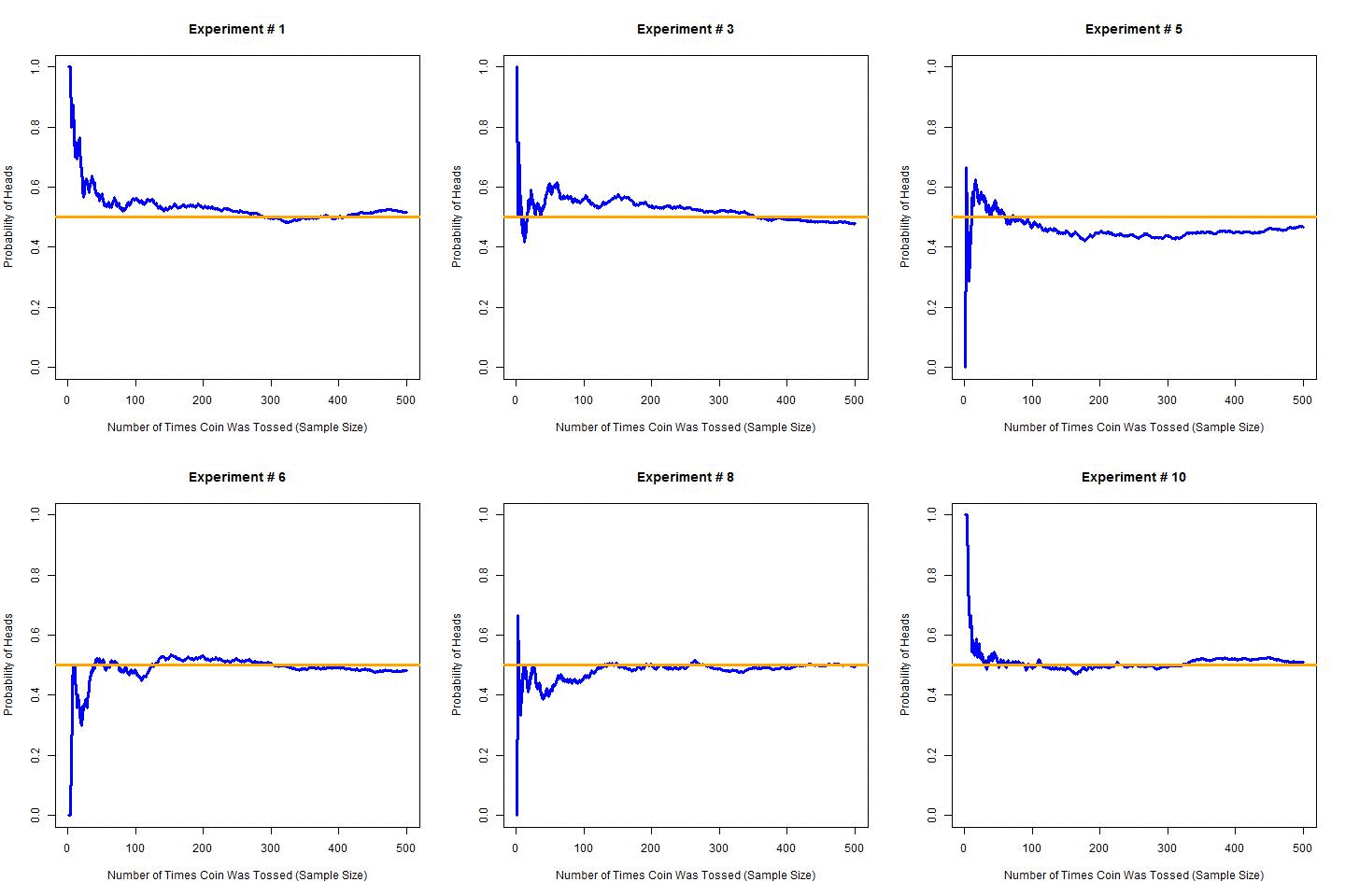
Now to extend the above experiment, I will perform 10 experiments with 500 tosses each and estimate probability at each step. I will simulate these experiments for the obvious reason that I don’t want to toss a coin 5000 times (i.e. 10 × 500 times). The following are the results of these simulations (R code for these simulations).
In this graph, the orange line is the actual probability i.e. 0.5, and the blue line is the estimated probability for each step. As expected the estimated probability is getting closer to actual probability with the increase in sample size (left to right).
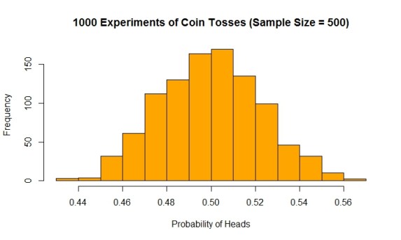
Now the question is how good is 500 as the sample size to estimate the probability of heads? For this, we will simulate 1000 experiments each with the sample size of 500, and estimate the probability of heads after each experiment. This histogram shows the estimated probability of 1000 experiments (R code for this simulation)
The histogram looks like a normal distribution or bell curve as would have expected from the central limit theorem (CLT) – we will come back to CLT in the next segment.
The summary statistics for this data:
| Min. | 1st Qu. | Median | Mean | 3rd Qu. | Max. | Std Dev. |
| 0.43 | 0.484 | 0.5 | 0.5006 | 0.5160 | 0.5620 | 0.0226 |
Both mean and median for 1000 experiments (sample size = 500) is close to 0.5. The standard deviation of these experiments is 0.0226. This standard deviation for multiple experiments is also known as the standard error of the estimate as we will learn later in this article.
We could have estimated the same values for mean and standard error through the theory suggested by the central limit theorem.
Central Limit Theorem & Sample Size
Let’s try to simplify the central limit theorem for our purpose of coin tossing. It states that mean of all the probabilities of heads estimated through all the experiments is equal to the actual probability of heads. In mathematical form, this is stated as:
We know that the actual probability of heads or π is 50%. Unlike this problem, for most practical problems the value of π is unknown. In such cases, we assume the probability obtained from experiment (p) as the expected probability.
For our one thousand experiments, we got the mean as 0.5006. Had we performed an infinite number of experiments we will have got an exact value for actual probability i.e. 0.5. But none of us has the time to do an infinite number of experiments. Only mathematicians can do these experiments in their heads but for all practical purposes, most of us can rely on simulations.
Another part of the central limit theorem states that standard error for estimation of proportions or probabilities is:
Here, π is the actual probability of heads for the fair coin which is 0.5. Hence, the standard error for a fair coin is:
In our simulated experiments, we got the standard error or standard deviation of estimated probabilities of heads:
The simulated results gave almost the same result as the theory suggested.
Identify the Right Sample Size
Now, let us come back to our original question for this article of identification of sample size. In the previous section, we have found the theoretical definition for standard error as:
We can reorganize the above equation to measure the value of n which is sample size.
Now, if you are OK with standard error as 10% of the actual probability of head (i.e. 10% of 0.5 i.e. 0.05). In this case, 95% of your results will be in the confidence interval of 0.4 to 0.6. This is calculated through 2 × standard error on either side of 0.5. A sample size of 100 will be good enough to achieve this confidence as shown in the calculation
On the other hand, if you want standard error as 0.5% of the actual probability of head (i.e. 0.005). In this case, 95% of your results will be in the confidence interval range of 0.495 to 0.505. However, to achieve this high level of precision the requirement of sample size is whopping 40000 tosses.
Hence, the entire sampling strategy is a trade-off between sample size and standard error. This table shows sample size requirement for the desired standard error as a percentage of probability of heads for a fair coin.
| Standard Error as % of Actual Probability of Heads (i.e. 0.5) | 20% | 10% | 5% | 2% | 1% | 0.5% |
| Standard Error | 0.1 | 0.05 | 0.025 | 0.01 | 0.005 | 0.0025 |
| Sample Size | 25 | 100 | 400 | 2500 | 10000 | 40000 |
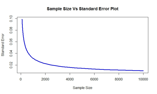
When we plot a sample size vs standard error plot, because of the inverse square relationship between them, toward the right side of the plot standard error doesn’t decrease as drastically as towards the left. This is an important concept to keep in mind while choosing the sample size for your analysis.

Sign-off Note
We have done the entire calculation of sample size based on the assumption that means is the measure that you want to estimate for a population. This is usually a good assumption for most analysis. However, it is always good for you to ask : is mean the right measure for your analysis? The right measure for your analysis depends on the question you are trying to answer.
For example, consider these two questions:
1. What is the salinity of the Pacific Ocean?
2. Is there another planet with intelligent life in the Universe?
In terms of population size, the number of drops in the ocean and planets in the Universe is similar. A couple of drops of water are enough to answer the first question since the salinity of oceans is fairly constant. On the other hand, the second question is a black swan problem. You may need to visit every single planet to rule our possibility of an intelligent form of life. Hence the sample size depends on the degree of similarity or homogeneity of the population in question.


Simple, crisp, to the point. Excellent!!
Roopam, thank you for a well-prepared and easy to read blog, I have been an often visitor here. Your style makes it easy to digest the information.
Knowing a bit about segmentation and machine learning, I wonder how well current algorithms can predict new Earth-like planets with just one sample in the training set (the Earth). Obviously, the chances increase with new planets, but again so far we have the only one.
Aleksandras, finding Earth-like planets is not exactly a machine learning problem, as you rightly mentioned, since there is not enough data. This is an ultra rare event and extremely sparse data problem and requires scientific and creative thinking. In my opinion, one of the ways to address this problem is identifying factors that are responsible for the presence of intelligent life form (assuming humans are intelligent 😉 ) on the planet. These are some of the factors I could think of: (I am making a few debatable assumptions here like all the life forms possible will be carbon based and the Earth is the only conducive condition in which life can evolve)
1) Proximity to Sun-like star
2) Presence of atmosphere
3) Presence of optimal ratio of carbon, nitrogen, and oxygen for carbon based lifeforms
4) Sustenance for enough year for intelligent form of life to evolve from primitive forms
The next task is to identify the presence of these conditions across the Universe to recognize planets where intelligent life-form can exist. This will make our search somewhat narrowed, and will not require us to visit all the planets.
Interesting and very easy to read and Understand.
Great Article Roopam,
Thanks,
Siddharth
Great Article Roopam. I am a regular reader of your blog.
Thanks
Hari