Painter and Time Series Decomposition – by Roopam

In the previous article, we started a new case study on sales forecasting for a tractor and farm equipment manufacturing company called PowerHorse. Our final goal is to forecast tractor sales in the next 36 months. In this article, we will delve deeper into time series decomposition. As discussed earlier, the idea behind time series decomposition is to extract different regular patters embedded in the observed time series. But in order to understand why this is easier said than done we need to understand some fundamental properties of mathematics and nature as an answer to the question:

Why is Your Bank Password Safe?

Mix one part of blue and one part of yellow to make 2 parts of green: a primary school art teacher writes this on the blackboard during a painting class. The students in the class then curiously try this trick and Voilà! they see green colour emerging from nowhere out of blue and yellow. One of the students after exhausting all her supplies of blue and yellow curiously asks the teacher: how can I extract the original yellow and blue from my two parts of green? This is where things get interesting, it is easy to mix things however it is really difficult (sometimes impossible) to reverse the process of mixing. The underlining principle at work over here is entropy (read the article on decision trees and entropy); reducing entropy (read randomness) requires a lot of work. This is essentially the reason why time series are difficult to decipher, and also the reason why your bank password is safe.

Cryptography, the science of hiding communication, is used to hide secrets such as bank passwords or credit card numbers and relies heavily on the above property of mixing being easier than “un-mixing”. When you share your credit card information on the internet it is available on the public domain for anybody to access. However, what makes it difficult for anyone without the key to use this information is the hard to decipher encryption. These encryptions at the fundamental level are created by multiplying 2 really large prime numbers. By the way, a prime number (aka prime) is a natural number greater than 1 that has no positive divisors other than 1 and itself. Now multiplication of two numbers, no matter how large, is a fairly straight forward process like mixing colours. On the other hand, reversing this process i.e. factorizing a product of two large primes could take hundreds of years for the fastest computer available on the planet. This is similar to “un-mixing” blue and yellow from green. You could learn more about cryptography and encryption by reading a fascinating book by Simon Singh called ‘The Code Book’.

Time Series Decomposition – Manufacturing Case Study Example

Back to our case study example, you are helping PowerHorse Tractors with sales forecasting (read part 1). As a part of this project, one of the production units you are analysing is based in South East Asia. This unit is completely independent and caters to neighbouring geographies. This unit is just a decade and a half old. In 2014 , they captured 11% of the market share, a 14% increase from the previous year. However, being a new unit they have very little bargaining power with their suppliers to implement Just-in-Time (JiT) manufacturing principles that have worked really well in PowerHorse’s base location. Hence, they want to be on top of their production planning to maintain healthy business margins. Monthly sales forecast is the first step you have suggested to this unit towards effective inventory management.

In the same effort, you asked the MIS team to share month on month (MoM) sales figures (number of tractors sold) for the last 12 years. The following is the time series plot for the same:

Now you will start with time series decomposition of this data to understand underlying patterns for tractor sales. As discussed in the previous article, usually business time series are divided into the following four components:

• Trend –  overall direction of the series i.e. upwards, downwards etc.
• Seasonality – monthly or quarterly patterns
• Cycle –  long term business cycles
• Irregular remainder – random noise left after extraction biof all the components 

In the above data, a cyclic pattern seems to be non-existent since the unit we are analysing is a relatively new unit to notice business cycles. Also in theory, business cycles in traditional businesses are observed  over a period of 7 or more years. Hence, you won’t include business cycles in this time series decomposition exercise. We will build our model based on the following function:

In the remaining article, we will study each of these components in some detail starting with trend.

Trend – Time Series Decomposition

Now, to begin with let’s try to decipher trends embedded in the above tractor sales time series. One of the commonly used procedures to do so is moving averages. A good analogy for moving average is ironing clothes to remove wrinkles. The idea with moving average is to remove all the zigzag motion (wrinkles) from the time series to produce a steady trend through averaging adjacent values of a time period. Hence, the formula for moving average is:

Now, let’s try to remove wrinkles from our time series using moving average. We will take moving average of different time periods i.e. 4,6,8, and 12 months as shown below. Here, moving average is shown in blue and actual series in orange.

As you could see in the above plots, 12-month moving average could produced a wrinkle free curve as desired. This on some level is expected since we are using month-wise data for our analysis and there is expected monthly-seasonal effect in our data. Now, let’s decipher the seasonal component

Seasonality – Time Series Decomposition

The first thing to do is to see how number of tractors sold vary on a month on month basis. We will plot a stacked annual plot to observe seasonality in our data. As you could see there is a fairly consistent month on month variation with July and August as the peak months for tractor sales.

Irregular Remainder – Time Series Decomposition

To decipher underlying patterns in tractor sales, you build a multiplicative time series decomposition model with the following equation

Instead of multiplicative model you could have chosen additive model as well. However, it would have made very little difference in terms of  conclusion you will draw from this time series decomposition exercise. Additionally, you are also aware that plain vanilla decomposition models like these are rarely used for forecasting. Their primary purpose is to understand underlying patterns in temporal data to use in more sophisticated analysis like Holt-Winters seasonal method or ARIMA.

The following are some of your key observations from this analysis:

1) Trend: 12-months moving average looks quite similar to a straight line hence you could have easily used linear regression to estimate the trend in this data.

2) Seasonality: as discussed, seasonal plot displays a fairly consistent month-on-month pattern. The monthly seasonal components are average values for a month after removal of trend. Trend is removed from the time series using the following formula:

3) Irregular Remainder (random): is the residual left in the series after removal of trend and seasonal components. Remainder is calculated using the following formula:

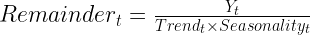
The expectations from remainder component is that it should look like a white noise i.e. displays no pattern at all. However, for our series residual display some pattern with high variation on the edges of data i.e. near the beginning (2004-07) and the end (2013-14) of the series.

White noise (randomness) has an important significance in time series modelling. In the later parts of this manufacturing case study. you will use ARIMA models to forecasts sales value. ARIMA modelling is an effort to make the remainder series display white noise patterns.

Sign-off Note

It is really interesting how Mother Nature has her cool ways to hide her secrets. She knows this really well that it is easy to produce complexity by mixing several simple things. However, to produce simplicity out of complexity is not at all straightforward. Any scientific exploration including business analysis is essentially an effort to decipher simple principles hiding behind mist of complexity and confusion. Go guys have fun unlocking those deep hidden secrets!