
Data Analytics Challenge – by Roopam
Sometimes answers lead to more questions. In data science this sometime is true almost everytime.
Analytics Challenge – The Shady Gamble
In the previous article, you were approached by Scotland Yard to investigate charges against a gambler with dubious character. The allegation against him was that he had loaded his die so that some numbers are more likely to appear after a throw than others. They were seeking your help to understand whether the gambler’s die is biased or not? They had shared the following barplot representation of the gambler’s previous 1000 throws.
| As mentioned in the previous part, all the analytics challenges on YOU CANalytics require your participation to proceed. We have some good discussion running in the comments section of the previous part (discussion link). This part will reveal a few more clues for you to further that discussion. I will use your comments from the previous part, along with some creative freedom, to move ahead with this investigation. |
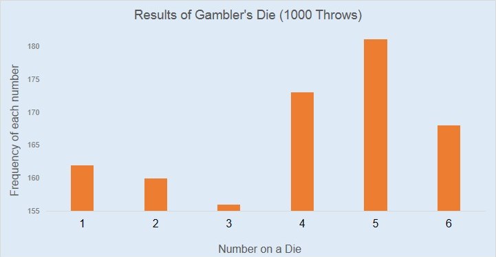
Your initial reaction after looking at this plot was : the gambler’s die looks biased. You know that for a fair die each number on the die has the equal likelihood of appearing. In other words, the length of all the bars in the above bar chart must be roughly the same. Since that doesn’t seem to be the case hence the die must be biased.
Later after a more careful analysis, you noticed that the bar plot is zoomed on the Y-axis. In this case, Scotland Yard has used Sherlock Holmes’ favorite instrument for detection i.e. magnifying glasses.
Realizing this, you make the appropriately-scaled version of the same plot (look this one starts from 0 on the Y-axis).

Please help Scotland Yard answer the following questions. Like the last time please add your comments in the discussion section at the bottom of this article.
| 1 | Do you still feel that the die is biased? Why or why not? |
| 2 | Is the use of magnifying glass (Sherlock Holmes’ favorite instrument for detection) justified here? Why or why not? |
| 3 | Could you see some similarity between this analysis and the way the popular press reports economic indicators (stock market in particular)? |
To continue with your analysis, you have placed the bars of expected values i.e. 1000/6 = 166.67 next to the observed value for the gambler’s die. The following is the same plot.
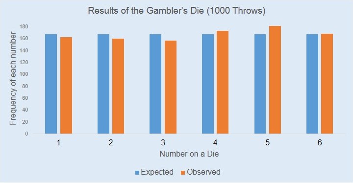
Now, our original question can be rephrased to: are the blue bars and the orange bars significantly different from each other? If yes then the coin is biased. At first, to answer this question you had suggested simulation. The idea behind simulation is to repeat the experiment of rolling 1000 trials of a die several times through a random number generator and compare those results with our observation.
Simulation is a good way to test our hypothesis however for this problem we will employ a much more theoretically robust method i.e. Chi-Square goodness-of-fit test. In it’s simplest form Chi-Square GOF is a normalized difference between expected and observed distributions, and comparing this difference against a standard value (i.e. Chi-Square distribution). Scotland Yard wants to know:
| 4 | What is the difference between simulation and Chi-square test? How are they similar to test random events? |
You wrote down the following lines of R code to calculate Chi-Square statistics (Credit for this code: Jason Corderoy / Ram). The first line of the code takes in observed value of frequency for each number on the die
Observed <- c(162,160,156,173,182,167)
The next line of the code produced expected frequency through uniform probability distribution where each number on the die has 1/6 chances of appearance.
Expected <- rep(1/6,6)
The subsequent line of the code does the Chi-Square goodness of fit test for observed and expected values.
test.chi <- chisq.test(Observed,p=Expected)
The final line of the code test the hypothesis at 0.05 significance level i.e. 5% chances that observed values are not the same as expected values.
ifelse(test.chi$p.value <= 0.05,
       "NULL Hypothesis Rejected: Die not fair.",
       "NULL Hypothesis not rejected: Die fair.")
After running the last line of code, R spews out the following result: “NULL Hypothesis is not rejected: Die fair.”. The inspector from Scotland Yard is completely confused by now. He phrased the following questions:
| 5 | What is the rationale behind choosing p-value of 0.05 as the threshold to accept or reject the hypothesis? |
| 6 | Is there a better way to represent the results rather than conclusive acceptance or rejection of hypothesis? How will it help? |
Finally, Scotland Yard provides you with one final piece of information around values that are in favor of the house. The house always makes money when a number above 3 appears on the die (Credit: Terry Taerum). The final question you hear from the inspector from Scotland Yard is:
| 7 | In the light of this new evidence i.e number 4,5 and 6 always make money for the house, would you change your conclusion about the die being fair? Why or why not? |
| This time, Scotland Yard has way too many questions for you (7 to be precise). You don’t need to discuss all of them, take your pick and start a discussion in the comment section at the bottom. Please mention the question number(s) in your comment. |
I think we can test it the same way although DF = 1 this time.
> actual = c(478,522)
> expected = c(1/2,1/2)
> test = chisq.test(actual, p=expected)
> ifelse(test$p.value test$p.value
[1] 0.1641035
For the earlier question about choosing the threshold for p-value, i am not aware of the history behind the threshold of 0.05 but my understanding is that as p value is basically about the odds of making a wrong decision, we can choose the value depending upon how lenient/strict we want to be
Please let me know if i am thinking in the right direction
Just wanted to reiterate that your blog is awesome. I learn a lot from your posts. Thanks
Missed this portion of the code (not used to ubuntu yet :))
ifelse(test$p.value <= 0.05, "Not Fair", "Fair")
Question 7: In the light of this new evidence i.e number 4,5 and 6 always make money for the house, would you change your conclusion about the die being fair? Why or why not?
The new evidence does not change the earlier conclusion that the die is fair.
We can treat this analogous to a coin toss.
Head: 4 or 5 or 6 (Total: 522)
Tail: 1 or 2 or 3 (Total: 478)
Using the test mentioned above by Rishab, the p-value for this case is 0.16. Hence we can not reject the null hypothesis that the die is fair.
Bonus answer:
Taking this a bit further, we see the boundary value where we can reject the fairness of the die.
chisq.test(c(heads=531,tails=469), p=c(.5,.5))$p.value
This will be < .05, hence we can reject the null hypothesis.
Question 7: In the light of this new evidence i.e number 4,5 and 6 always make money for the house, would you change your conclusion about the die being fair? Why or why not?
I do not profess to be an expert at this but I would just like to lay down my thoughts and would appreciate feedback if there are any gaping holes in my logic from those more experienced that myself.
I find it convenient for the house that all 4:6 die rolls occured above expectation whereas 1:3 were all below expectation. It just feels fishy to me. This ties in nicely to Terry Taerum’s point in clue 1 that “in money laundering, the objective is to make the “whole appear whole” while burying the bias.”
So I decided to run a random sample of 5,000 instances of 1,000 dice throws and look at the probabilty of hitting 4:6 all above expected frequency whilst 1:3 occured below expected frequency.
When I run the below code I get a 2.94% (roughly 1 in 34) chance that all the numbers favouring house (4:6) occur above expected frequency whilst rolling 1:3 all occur below expected frequency.
It feels more likely that the dice is in fact bias when I look at it in this way. Perhaps biasing 3 numbers instead of just 1 or 2 means bias can go undetected by Chi Squared methods?
The R code I use to simulate 5,000 instances and get the 2.94% probability is:
set.seed(12345)
samp <- sample(c(1:6),1000,replace=TRUE)
all.samples <- as.numeric(table(samp))
all.samples (1000/6)),ncol=6)
all.samples <- as.data.frame(all.samples)
names(all.samples) <- c("One","Two","Three","Four","Five","Six")
for (i in 1:(5000-1)) {
samp <- sample(c(1:6),1000,replace=TRUE)
this.sample <- data.frame(table(samp))$Freq
this.sample (1000/6)),ncol=6)
this.sample <- as.data.frame(this.sample)
names(this.sample) <- c("One","Two","Three","Four","Five","Six")
all.samples <- rbind(all.samples,this.sample)
}
actual.occurences <- nrow(subset(all.samples,One == 0 & Two == 0 & Three == 0 & Four == 1 & Five == 1 & Six == 1))
observed.prob <- actual.occurences/5000
observed.prob
My apologies not sure what happened but my code posted above is wrong. Use this instead:
set.seed(12345)
samp <- sample(c(1:6),1000,replace=TRUE)
all.samples <- as.numeric(table(samp))
all.samples (1000/6)),ncol=6)
all.samples <- as.data.frame(all.samples)
names(all.samples) <- c("One","Two","Three","Four","Five","Six")
for (i in 1:(5000-1)) {
samp <- sample(c(1:6),1000,replace=TRUE)
this.sample <- data.frame(table(samp))$Freq
this.sample (1000/6)),ncol=6)
this.sample <- as.data.frame(this.sample)
names(this.sample) <- c("One","Two","Three","Four","Five","Six")
all.samples <- rbind(all.samples,this.sample)
}
actual.prob <- nrow(subset(all.samples,One == 0 & Two == 0 & Three == 0 & Four == 1 & Five == 1 & Six == 1))
actual.prob/5000
It’s not pasting all the copied text… So weird.
Just replace 4th line of code:
all.samples (1000/6)),ncol=6)
with:
all.samples (1000/6)),ncol=6)
Sorry for clogging up the comments.
Hopefully it works this time…
all.samples = matrix(as.numeric(all.samples>(1000/6)),ncol=6)
If not I give up.
Hi Jason,
I read somewhere that the Hosmer Lemeshow test is not a very good GOF test as result depends on number of groups you segregate the data into (and the results vary).
Now essentially, if we group 1,2,3 and 4,5,6 then we are in effect doing the same thing. Hence it’s possible that chi-square is not be the right way to judge the dice
Can anyone please explain the reason for discrepancy in hosmer lemeshow test? Also which test is universally acceptable for categorical data?
One other question that i have is:
In your code, you have created an indicator based on uniform distribution (167 for each no) and then calculated the probability. Consider 2 hypothetical cases:
159,159,159, 161,161,161 vs. 100,100,100,233,233,234. Both these cases will be counted as equal in your analysis but shouldn’t the analysis be weighted based on deviation from the mean.
Please let me know if this makes sense. Thanks
Hi Rishabh,
Regarding you comment “Both these cases will be counted as equal in your analysis but shouldn’t the analysis be weighted based on deviation from the mean.” I agree with you but feel the need to return to Chi Square.
The Chi-Square statistic did not reject the null hypothesis. This test takes into account variance between observed and expected observations by taking the ‘sum of (Actual probability-expected probability)^2/expected probability’ in determining whether we exceed or match the critical Chi Squared value.
This is why I looked at the 1/0 re-grouping of each number seeing as Chi-Square seemed to hit a dead end.
What I find most interesting is –
say the observed rolls were this:
Observed <- c(162,160,156,173,82,267)
instead of this:
Observed <- c(162,160,156,173,182,167)
The house still makes the same winnings (assuming equal pay for 4,5 and 6) but now there is 100 less 5s and 100 more 6s. So a 1/0 grouping of 1:3/4:6 wouldn't pick this up.
But P-Value would change considerably:
Observed <- c(162,160,156,173,82,267)
Expected <- rep(1/6,6)
test.chi <- chisq.test(Observed,p=Expected)
test.chi$p.value
All the way down to .30949e-21 <- way below 0.05 although house would be making same profit (assuming equal payout on 4,5 and 6 of course).
This is the part I find interesting. It seems to be in the houses advantage to spread fairly evenly above frequency expectations on numbers 4, 5 and 6 instead having any one of these get too many or too few rolls.
Hi Jason,
It appears that you are overly restrictive in selecting the favorable occurrences.
How about running your simulation after replacing your subset with this subset?
actual.prob <- nrow(subset(all.samples,One + Two+ Three < Four + Five + Six))
(This might not be the right subset, but it is less restrictive than your selection. ie., it selects more cases compared to your selection).
Excellent point Ram,
I just thought the 1:3 v 4:6 distribution to be a tad sus. I thought that optimally the house would get 4+ above expectation and 1-3 below expectation perhaps just enough to hide bias. But it doesn’t appear to me that that’s a good finding in itself to support any conclusion. Just a hunch really.
The only reason I’ve gone down this rabbit hole is assuming that if casino’s cheat then they would make it undetectable if possible and somewhere far from easily detectable and as close as possible to undetectable in reality. So why not be a tad suspicious of all 4+(3-) rolls hitting at a frequency above(below) expectation?
I’ll follow this path I’ve started walking on for better or worse for now. I’m thinking if in fact there is some bias toward higher numbers (>3) then what if we simulate the observed dice distribution assuming there’s instead 2 identical dice? This would instead see if rolling 2 dice with each simultaneously hitting >3(<=3) significantly more (less) than expected effectively compounding any subtle bias that may exist in the dice. Then test if p-value is significant.
Chi-Square on 2 identical dice – each with same distribution as provided in problem:
set.seed(12345)
Observed <- c(rep(1,162),rep(2,160),rep(3,156),rep(4,173),rep(5,182),rep(6,167))
Observed.2Dice <- matrix(sample(Observed,1000*2,replace=TRUE),ncol=2)
observed.probs <- prop.table(table(apply(Observed.2Dice,1,sum)))
observed.sum <- table(apply(Observed.2Dice,1,sum))
expected.probs <- prop.table(table(apply(expand.grid(1:6,1:6),1,sum)))
test.chi <- chisq.test(observed.sum,p=expected.probs)
test.chi$p.value
We now get a P-Value of 0.018.
Expected (Observed) proportions are:
2: 0.03 (Observed = 0.02)
3: 0.06 (Observed = 0.04)
4: 0.08 (Observed = 0.09)
5: 0.11 (Observed = 0.10)
6: 0.14 (Observed = 0.12)
7: 0.17 (Observed = 0.17)
8: 0.14 (Observed = 0.16)
9: 0.11 (Observed = 0.11)
10: 0.08 (Observed = 0.09)
11: 0.06 (Observed = 0.08)
12: 0.03 (Observed = 0.03)
^ all 2:6 rolls are below expectation whilst all 8+ rolls are above expectation
So maybe compounding subtle bias (e.g. simulate 2 dice) is the only way to detect subtle bias?
Maybe I'm way off. I would just find it hard to believe that casino's would cheat without first designing bias that could go undetected provided small sample sizes using Chi Square.
I repeat the only reason I've gone down this rabbit hole is assuming that if casino's cheat then they would make it undetectable if possible and somewhere far from easily detectable and as close as possible to undetectable in reality. So why not be a tad suspicious of all 4+(3-) rolls hitting at a frequency above(below) expectation?
Another option:
Ask for more data. If we analyze 5000 or 10000 throws, we will get a more definitive answer.
That would solve all our problems. Assuming the exact same distribution over 10,000 throws chi test p-value = 0.000049… Case closed.
With only 1,000 throws at least we have the opportunity to get a little creative 🙂
Fair enough.
If we have to work with 1000 throws, here is another option:
Divide the 1000 throws chronologically into 5 groups so that each group contains 200 throws. (Currently, we are not given data from individual throws, Scotland Yard will have to get this data from the casino).
Run separate tests on each group of 200 throws..
Do you find 4,5,6 getting the higher share in each group?
If yes, it will support the case that the die is rigged.
Basically if we keep the distribution constant and vary the number of observations, we come to a different conclusion about the dice.
One fundamental questions that i have is: Assume we have a very (very) high no of data points, we can look at the total count of (1,2,3) & (4,5,6), and if the count deviates from total count/2 we can say that the dice is biased. Now in our current scenario(s) we can’t just look at the distribution because the data points are few. Hence we use statistics (chi-square) to determine the bias for us. Now if even chi-square results depend on the number of throws, then it doesn’t seem to be a very solid test (to me).
Does this make sense?
Ram and Rishabh,
I think that your idea is excellent. Get data on each die roll and if the 4:6 higher frequency distribution is consistent in each (or majority of?) of the 5*200 samples then that would point toward bias. We may even want to chunk into 50 and 100 rolls per group also and then compare results. See if there’s consistency in findings amongst smaller and larger groups. Maybe this could strengthen evidence for or against our findings?
Rishabh, the fact that Chi-Square P-Value does vary based on sample size is a good thing. E.g. throwing a coin twice and hitting heads twice v throwing coin 1,000 times and hitting heads 1,000 times shouldn’t be ignored. Same goes for dice throws. We get this intuitively so it’s nice that Chi-Square also also does. It just gets much muddier when we are talking bigger numbers. Our human minds find it harder to picture exactly what’s causing a significant P-Value at say 10,000 throws but not at 1,000 throws given this probllems dice distribution.
So in line with what you mentioned if given more data points and if 4:6 rolls deviate >+1.96 SD’s from the means (assuming significance level of 0.05) then we could reject null hypothesis. Although I point out below that givne casino’s financial motivation to cheat then are we willing to be a little flexible on P-Value significance level? What if we get P-Value of 0.051 or 0.06 for example?
5. The value for which P=0.05, or 1 in 20, is 1.96 or nearly 2; it is convenient to take this point as a limit in judging whether a deviation ought to be considered significant or not. Deviations exceeding twice the standard deviation are thus formally regarded as significant. Using this criterion we should be led to follow up a false indication only once in 22 trials, even if the statistics were the only guide available. Small effects will still escape notice if the data are insufficiently numerous to bring them out, but no lowering of the standard of significance would meet this difficulty- Fisher (the famous one)
Thanks Shailesh,
I’ve now learned more about the history of P-Values after also reading a few more articles online. And there’s no hard-fast rule although 1 in 22 false positives sure is a nice default 🙂
We should consider the problem at hand and financial incentive for a casino to cheat in determinnig P-Values?
E.g. if you are drinking an immortality liquid you may accept a 50% chance of sudden death given a 50% chance of immortality.
You wouldn’t accept the odds of 50% death if it were just Coca Cola though I assume. Seeing as the benefit would only be a tasty drink. Not worth risking death for.
If cheating was no benefit to a Casino then surely attempting to detect cheating would be less meaningful but given incentive to cheat would that not imply that we should be more flexible toward a higher P-Value than a lower P-Value?
6. is it about famous Fisher’s and Neyman-Pearson theories?
For q 7…
we can create 2 group
Group A (1,2.3)
Group B (4,5,6)
And then do a F test for significance….
This shud give, whether the errors is because of chance or because Die is unfair.
do share your inputs on this,
Here is a real-life incident akin to the casino puzzle. This might help us understand the logic:
A local school has 810 students: 430 boys and 380 girls.
Recently the school had to select a team for an inter school competition.
After screening the students, the school came up with a short-list with 8 boys and 12 girls.
One parent, after seeing the list complained that the boys are under-represented in the team, and it is unfair to the boys.
Does his complain have merit?
Regarding choosing a value for alpha, the Type 1 Error rate. I like to think of it as trying to strike a balance between risk and consequences (mental picture: teeter-totter). The greater the consequence of being wrong, the lower the risk one should assume – and vice versa. Remember, we are trying to find signals in the data – if they exist. The lower alpha is, the greater beta is, and the lower the Power is – and Power is the probability of detecting a signal if it exists.
Informative post but too complicated.