Data! data! data!” he cried impatiently. “I can’t make bricks without clay.
– Sherlock Holmes

Sherlock Holmes : Data Analytics Challenge – by Roopam
In this article, we are starting a new series on YOU CANalytics that can’t proceed without your participation to solve the data analytics mysteries. In the beginning of each article of this series, you will get a problem that needs you to analyse data.Subsequent articles after the first article will reveal clues based on your questions and comments. Mystery challenges on this series will vary from easy to very hard.
All the analytics challenges will have the same pitfalls we experience in real-world business analytics. Also, like most real problems there are no wrong answers here. So wear your Sherlock Holmes cap, lift your magnifying glass, and get started. Please do write your questions, comments, solution approaches, opinions, thought processes, answers etc. in the discussion section at the bottom of this page.

Analytics Challenge 1 : The Shady Gambler
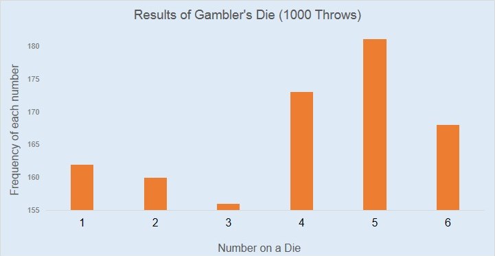
 They all say he is a crook. He has ruined many lives by the use of his die. The allegation against him is that he has loaded his die so that some numbers are more likely to appear after a throw than others. After numerous complaints, Scotland Yard has approached you to investigate the results of the gambler’s use of a die. The following is a bar plot representation of the previous 1000 throws through which he has made a good fortune for his gambling house. Have a look at it and suggest if the allegations against him are correct.
Analyse the above plot and tell whether the gambler’s die is biased or not? In the process, you may want to share your opinion on deeper questions such as: what is randomness and how to measure it?
| Please share your comments, solution approaches, opinions, thought process, answers, and suggestions for this problem at the bottom in the Leave a Comments section. You could ask for more information and Scotland Yard will try to provide it to you. |
Approach:
1. Simulate 1000 throws. In excel use the =randbetween(1,6) function to randomly choose a number from 1 to 6 as the winning throw. Calculate the probabilities for 1 to 6 by averaging across the 1000 simulated throws. Calculate mean and std deviation of these 6 probabilities.
2. Simulate point 1 several times maybe 100 times, and take the average of mean and std deviation. These figures will be a good indicator of the distribution of the probabilities
3. Calculate the probabilities from the alleged cheating gambler’s past 1000 tries. Calculate mean and std deviation. Compare it with our simulated values to draw inference whether they are same or different by ANOVA.
Thanks Manish for you comment. Chi-square test is a better appropriate approach here, check out the following link CLUE # 2.
The gambler’s throw of the die is not random. Assuming the die to be a fair die, The chances of seeing all 6 numbers should be equi-probable and should follow a uniform distribution.
Hi Vaishnavi, thank for sharing your ideas, though you may want to reconsider your response. Let us know what you feel in the new light of evidence CLUE # 2.
There is some evidence that the dice is loaded and not random.
Reasoning:
The frequency of the 1,2,3,4,5,6 is taken as 162,160,156,173,182,167 as given in the bar plot. The mean value is 166.67 and the population std deviation is 9.54.
The ideal distribution should be 166.67 for each number to total up to 1000 for an unbiased dice.
Here, the sample size is 1000 and hence the std dev of the sampling distribution will be = pop std dev /sqrt(sample size) = 9.54/sqrt(1000) = 0.3
Now we calculate the z-score for the frequency of each number using the following formulae :
(freq of the the number out of 1000 – ideal freq of the number )/std dev of sampling distribution
Z-scores :
1 : (162-166.67)/0.3 = -15.46
2 : (160-166.67)/0.3 = -22.09
3 : (156-166.67)/0.3 = -35.34
4 : (173-166.67)/0.3 = 20.98
5 : (182-166.67)/0.3 = 50.81
6 : (167-166.67)/0.3 = 1.1
So, here you can see that only the number 6 has a z-score (1.1 <1.96) which falls within the confidence interval of 95% of an unbiased dice. Z-scores of the remaining numbers are very high.
Conclusion: In the given sample of 1000 observations, numbers from 1- 5 have frequency values which have very low chance of happening in an unbiased dice.
Kinjal,
It seems that you are using incorrect std. dev. to calculate the z score. That is why you are getting such incredibly high z scores.
If you divide by the std. dev. of population, you will get reasonable z scores for all the 6 counts.
Good one Roopam.
The allegation has no merit and it cannot be accepted.
Manipulation of axis range.This is a common trick used to mislead unsuspecting readers.
Here is a code segment in R to simulate 1000 throws of a fair die and plot the results:
############
library(lattice) # this is for the barchart.
s1=sample(1:6,1000,replace=T) # simulate 1000 throws
table(s1) # shows the distribution of values 1 thru 6
barchart(table(s1),horizontal=F) # the distribution looks fair
### Now run this code to redraw the bar chart.
barchart(table(s1),ylim=range(table(s1)),horizontal=F) # Does the distribution look fair?
Execute the code segment several times and inspect the plots.
You will conclude that the gambler is not shady at all.
the question is not whether the distribution of the throws are random but whether the dice is unbiased. And it clearly looks like the dice is biased.
We cannot be sure if its random event or not with the given data. We need more data for e.g. can you publish the round details assuming a round be made up of sequence of 10 throws. 1000 throws would mean 100 rounds.
That’s a good point, the question is : whether the die is biased or not? Thanks for pointing that out.
Sangram,
1. Do you consider the die to be unbiased ‘if and only if’ the counts are identical?
example: 166,167,166,167,167,167
2. Will you consider the die to be biased if the counts are as below?
a. 170,163,168,165,166,164 OR
b. 180,153,169,164,166,164
In my opinion, all of the above 3 are examples of unbiased die throws. As Rishab has pointed out, you can test this using the chisquare test.
If i consider only 10 throws, then there is a 1/(6)^10 probability that 6 will occur 10 times but it can happen. Theoretically the best way in my mind to find out whether the dice is biased or not is to get a very large sample and see the distribution. 1000 in my opinion is too small a sample to judge the dice based on just the distribution
To understand the concept, perhaps we can use the analogy of a coin toss.
If I toss a coin 1000 times and get:
500 Heads and 500 Tails, we conclude that the coin is fair.
499 Heads and 501 Tails, can we conclude that the coin is fair?
490 Heads and 510 Tails, can we conclude that the coin is fair?
410 Heads and 590 Tails, can we conclude that the coin is fair?
We can also do a chi square test to determine whether the dice is fair or not (with DF = 5)
Thanks Roopam,
Loved the puzzle. I’m really looking forward to the next one. Best way to learn is to do and this really motivates the doing.
I get: Die fair based on Chi Square test with confidence interval of 0.05.
R Code:
actual <- c(162,160,156,173,182,167)
expected <- rep(1000/6,6)
prob <- rep(1/6,6)
df <- as.data.frame(rbind(actual,expected))
names(df) <- as.character(1:6)
test.chi <- chisq.test(df)
ifelse(test.chi$p.value <= 0.05,"NULL Hypothesis Rejected: Die not fair.","NULL Hypothesis not rejected: Die fair.")
Thanks Jason, I am also enjoying reading all the comments. We have all made a good collective start here. There are many more puzzles to follow – so please stay tuned.
However I must point out, this puzzle by no means is over. To me, all the easy puzzles are usually the most intriguing since there are so many layers to them and each layer makes us jump into an unexplored depth.
Also, thanks for sharing your R code. I will use a variant of your code in the next part.
Hi Jason,
Thank you for the posting the code.
It looks like your parameters for chisq.test are incorrect, (Your test gives a p-value .93).
Instead, try this code:
test.chi <- chisq.test(actual, p=prob)
test.chi$actual
test.chi$expected
##For this test, you will get a different p value .74.
Here is a nice tutorial:
http://ww2.coastal.edu/kingw/statistics/R-tutorials/goodness.html
Thanks a tonne Ram,
That makes a lot of sense now.
So updated code would be:
actual <- c(162,160,156,173,182,167)
prob <- rep(1/6,6)
test.chi <- chisq.test(actual, p=prob)
test.chi$expected
test.chi$observed
test.chi$p.value
# P-Value of 0.74 as stated by Ram.
When we run both a Chi-Square and Normality test, we get p- vale > 0.05, so the dice is unbiased.It’s a fair dice. Starting Y-axis from 155 is to create confusion.
The quick and dirty is to do a Chi Squared of observed against expected (166.67) resulting in an overall test which (as has been pointed out) is not significant. However, those of us who have been around the block a few times realize that in money laundering, the objective is to make the “whole appear whole” while burying the bias. So (since I have enough statistical sense to not gamble) I’d need to know what values are in favor of the house and if 1000 throws are needed for the house to make money.
in other words (to reply to myself)…. skimming requires very small profit (e.g. the slot machines)… what is the “bias” required in order for the house to show a profit and what is sufficient to be considered a profit…
Excellent point Terry! You have questioned some fundamental and widely accepted beliefs of statistical inferences such as significance level and p-values. Why do we use 0.05 as the standard? Are we missing the forest for the trees in the process?
Let’s explore this more when the new set of clues (around incentives for the house) will come our way in the next parts of this article. I am sure everyone here would love to hear more from you on this subject.
Hi Roopam… thanks – as an aside you should know I follow quite a bit of what you do and I think it is generally brilliant, thoughtful, insightful – and entertaining. I look forward to your contributions.
Thanks Terry, good to hear such kind words.
You certainly have a great body of work in analytics, and I look forward to hear more from you in this series of articles.
We can approach this problem using concept of information theory also.
Let us consider an was unbiased die, so for every number in 1000 trials expected mean should be 166.66
Entropy,H(random)= (6 x 166.67/1000) x log2(1000/166.67)= 2.5854
Now, for the die of the gambler
Entropy.H(test)= sum_i=1_to_6_[-p(i)log2(p(i))] = 2.5832
Since the difference in entropies is not significant, we don’t have enough evidence to say that the die is biased.
Regarding the terminology used:
1) The six frequencies will yield the standard deviation of the *sample* – not the population. The sample standard deviation is only an estimate of the population standard deviation.
2) Dividing the sample standard deviation by the square root of the sample size gives an estimate of the standard deviation of the distribution of *averages* of groups of 1000.
thank you for your sharing ideas