---

If you want to gain a sound understanding of machine learning then you must know gradient descent optimization. In this article, you will get a detailed and intuitive understanding of gradient descent to solve machine learning algorithms. The entire tutorial uses images and visuals to make things easy to grasp.

Here, we will use an example from sales and marketing to identify customers who will purchase perfumes. Gradient descent, by the way, is a numerical method to solve such business problems using machine learning algorithms such as regression, neural networks, deep learning etc. Moreover, in this article, you will build an end-to-end logistic regression model using gradient descent. Do check out this earlier article on gradient descent for estimation through linear regression 

But before that let’s boldly go where no man has gone before and explore a few linkages between…

Gradient Descent & Star Trek

Star Trek is a science fiction TV series created by Gene Roddenberry. The original show was first aired in the mid-1960s. Since then Star Trek has become one of the largest franchises for Hollywood. Till date, Star Trek has seven different television series, and thirteen motion pictures based on its different avatars.

The original 1960s show is among the first few TV shows I remember from my childhood. Captain Kirk and Spock are cult figures. The opening line of Star Trek still gives me goosebumps. It goes like this:

Space, the final frontier. These are the voyages of the starship Enterprise. Its five-year mission: to explore strange new worlds, to seek out new life and new civilizations, to boldly go where no man has gone before.

– Opening Dialogue, Star Trek

Star Trek is about exploring the unknown. Essentially, trekking as a concept is about making a difficult journey to arrive at the destination. You will soon learn that gradient descent, a numeric approach to solve machine learning algorithm, is no different than trekking.

Moreover, Star Trek has this fascinating device called Transporter – a machine that could teleport Captain Kirk and his crew members to the desired location in no time. Keep the ideas of trekking and Transporter in your mind because soon you will play Captain Kirk to solve a gradient descent problem. But before that let’s define our business problem and solution objectives.

Market Research Problem – Logistic Regression

You are a market researcher and helping the perfume industry to understand their customer segments. You had asked your team to survey 200 buyers (1) and 200 non-buyers (0) of perfumes. This information is stored in the y variable of this marketing dataset. Moreover, you have asked these surveyees about their monthly expenditure on cosmetics (x₁ – reported in 100) and their annual income (x₂ – reported in 100000). In this plot, you plotted these 400 surveyees on the x₁ and x₂ axes. Moreover, you have marked the buyers and non-buyers in different colors. You can find the complete code used in this article at Gradient Descent – Logistic Regression (R Code).

Clearly, the buyers and non-buyers are clustered in separate areas of this plot. Now, you want to create a clear boundary or wall to separate the buyers from non-buyers. This is kind of similar to the wall Donald Trump wants to build between the USA and Mexico. You could still see some Mexicans on the American territory and vice-a-versa.

Another representation of this wall is the density plot as shown below. Notice, in this plot, we have taken both x₁ and x₂ collectively as x₁ + x₂. The reason why we could do this because the data was prepared in such a way to simplify things.

As you may have noticed, if you divide this graph in half at x₁ + x₂= 140 then on the right-hand side you predominantly have the buyers. Also, the left-hand side has more non-buyers then buyers. However, there is still a bit of infringement of the buyers into the non-buyers’ territory and vice-a-versa.

A better representation would be to divide the territories fuzzily or probabilistically to incorporate both cultures and set of people. This is precisely the point all the political leaders like Donald Trump miss. This is possibly also the reason we have territory problems like Gaza Strip, Kashmir etc.

Logistic Regression Equation and Probability

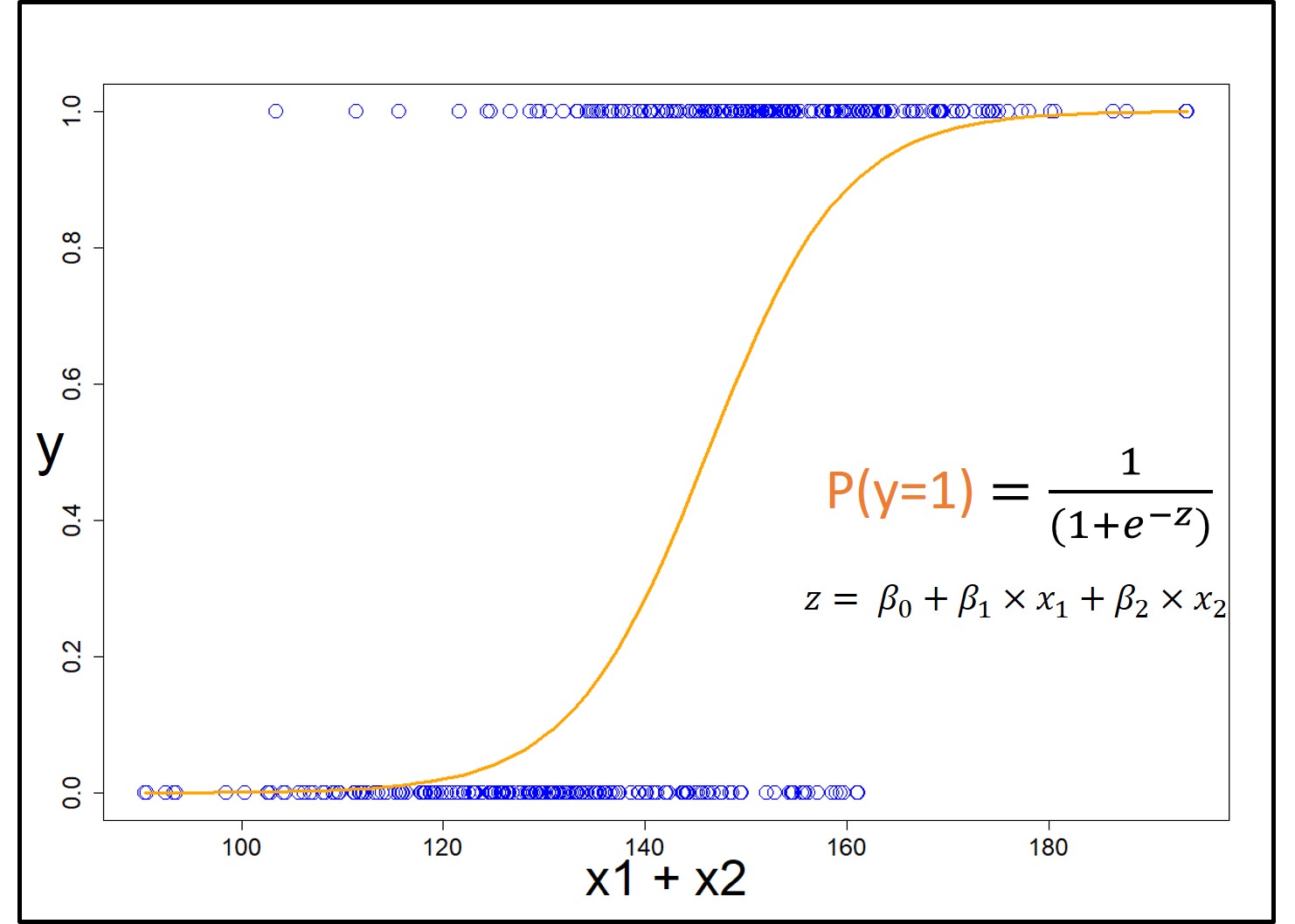
Mathematics, however, allows data to mingle and live in better harmony. To discover this, let’s plot y as a function of x₁ + x₂ in a simple scatter plot. Don’t forget y=1 is for the buyers of perfumes and y=0 is for the non-buyers.

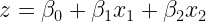
The reason we have plotted this bland looking scatter plot is that we want to fit a logit function P(y=1) = to this dataset. Here, P(y=1) is the probability of being a buyer in the entire space of x₁ + x₂. Moreover, z is a linear combination of x1 and x2 represented as .

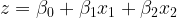In addition, for simplicity, we will assume β₁ = β₂ . This is not a good assumption in a general sense but will work for our dataset which was designed to simplify things.

Now, all we need to do is find the values of β₀ , β₁ and β₂ that will minimize the prediction errors within this data. In other words, this means we want to find the values of β₀ , β₁ and β₂ so that most, if not all, buyers get high probabilities on this logit function P(y=1). Similarly, most non-buyers must get low probabilities on P(y=1).

The quest for such β values is the job of gradient descent. Like other quests, as you will soon see, this requires a long journey and lots of walking.

Gradient Descent Optimization and Trekking

Gradient descent works similar to a hiker walking down a hilly terrain. Essentially, this terrain is similar to error or loss functions for machine learning algorithms. The idea with the ML algorithms, as already discussed, is to get to the bottom-most or minimum error point by changing ML coefficients  β₀ , β₁ and β₂ . The hilly terrain is spread across the x, and y-axis on the physical world. Similarly, the error function is spread across coefficients of machine learning algorithm i.e. β₀ , β₁ and β₂ .

The idea is to find the values of the coefficients such that the error becomes minimum. A better analogy of gradient descent algorithm is through Star Trek, Captain Kirk, and Transporter – the teleportation device. I promise you will get to say “Beam Me Up, Scotty” the legendary line Captain Kirk use to instruct Scotty, the operator of Transporter, to teleport him around.

Captain Kirk to Solve Gradient Descent

Assume you are Captain Kirk. A wicked alien has abducted several crew members of the Starship Enterprise including Spock. The alien has given you the last chance to save your crew if only you can solve a problem. The problem involves finding the minimum value of the variable y for all the possible values of x between -∞ to ∞.

Now, you are Captain Kirk and not a mathematician so you will use your own method to find the minimum or lowest value of y by changing the values of x. You have found a landscape in the exact shape of the function with x and y-axes that spreads across the Universe. You will ask Scotty to teleport you to a random location on this landscape and then you will walk down the landscape to find the value of x that will generate the lowest value of y. By the way, y here is similar to the error function and x is similar to the ML coefficients i.e β values.

Now all of us humans, including Captain Kirk, can figure out which way is the downward slope just by walking. It takes a lot more effort to walk upwards than downwards. We could also figure out a flat plane because the effort is same no matter which direction you walk. In the landscape Captain Kirk is walking, there are just 5 flat points with A, B, and C as the 3 bottom points. However, the problem with this terrain is that there are three minimum values – here A and B are the local minima. C, on the other hand, is the global minimum or the lowest value of y at x=3. Different locations that Captain Kirk starts by being beamed at random will settle him at different minima since he will only walk down.

We will come back to this problem of local minima, but before that let’s identify the mathematical equivalent of walking up or down which the actual gradient descent optimization will use.

Gradient Descent and Differential Calculus

The mathematical equivalent of human ability to identify downward slope is differentiation of a function also called gradients. The differentiation of the landscape Captain Kirk was walking is:

 

Now, if you insert x=3.1 in this equation you will get the as 4.83. The positive value indicates it’s an upslope ahead. This mean Captain Kirk, or the pointer for gradient descent algorithm, needs to walk backward or toward the lower values of x. Similarly, at x=2.9,  the = -3.27. The -ve value means it is a downslope ahead, and Captain Kirk will walk forward or towards the higher values of x.

At x=3, the global minima,  =0. This means there is no slope or you have reached a flat plane. As it turns out, the above polynomial equation can be simplified to this. It was a trick question from the alien.

We can find minimum values of this function without gradient descent by equating this equation to 0. =0 for, x = -2, -1, 1, 2, and 3. So, if Captain Kirk knew some math he could have avoided all the walking.

Let’s use this knowledge to find the machine learning prediction solution to our market research data.

Solution – Logistics Regression

In the market research data, you are trying to fit the logit function to find the probability of perfume buyers P(y=1). We don’t want to write P(y=1) many times hence we will define a simpler notation : P(y=1)= .

We also  know that z in the above equation is a linear function of x values with  β coefficients i.e.

Now, to solve this logit function we need to minimize the error or loss function with respect to the β coefficients. The loss function ( ) for a logistic regression problem is:

This loss function ( ) is cleverly designed to make the problem a convex optimization problem which is a fancy way to say that the function is like a bowl. Like a bowl, this function has just one base or global minimum value and there are no local minima. This plot shows the loss function for our dataset – notice how it is like a bowl. This convex function has solved a big problem that Captain Kirk faced of having several local minima.

Remember, for simplicity, we are assuming β₁ = β₂ in the above plot so that we could use x₁ and x₂ collectively as x₁ + x₂. The data was also prepared to keep this assumption but despite this, the real β₁ and β₂ will have different values if you will solve for independent x₁ and x₂.

Getting to the bottom

Now, you want to solve logit equation by minimizing the loss function by changing β₁ and β₀. To identify the gradient or slope of the function at each point we need to identify the derivatives of the loss function with respect to β₁ and β₀. Since we assumed β₁ = β₂ we are essentially working with one variable (x₁ + x₂) instead of two (x₁ & x₂).

It turned out that derivatives are simply (I have shown the derivation of this at the bottom of this article after the Sign-Off Note – and trust me these results are not that difficult to derive so do check them out) :

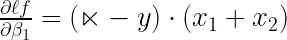
and,

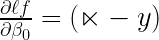
By using these values you can now send Captain Kirk to find the bottom of this loss function bowl. Also, while running the gradient descent code it is prudent to normalize the x values in the data. This will reduce Captain Kirk’s walking time or make the algorithm run faster. It turned out that the loss function bowl has the bottom at β₀ = -0.0315 and β₁ = 2.073 for normalized x1+x2 values.

 

The normalized x₁+x₂ value β values can be easily modified to actual values of x₁ and x₂ and in that case non-normalized β₀ = -15.4438 and β₁ = 0.1095. I will leave it up to you to figure out the logic of denormalizing the β values.

If you will run the gradient descent without assuming β₁ = β₂ then β₀ =-15.4233,  β₁ = 0.1090, and β₂ = 0.1097. I suggest you try all these solutions using this code: Gradient Descent – Logistic Regression (R Code).

Sign off Note

The original script of the Star Trek series was written without the mention of Transporter or the teleporting device. It was later realized that the lower budget of the show would not allow filming of the starship landing on unknown planets. They then devised a smaller vessel ship that was also beyond the budget of the show. Finally, a low-cost teleportation device (Transporter) was conceived. Thank heavens for the low-budget creativity because of which we have Transporter – a fascinating device!

Derivation of Gradients for Gradient Descent Function

You just need to know the following four basic derivatives to derive the lowest value of the loss function i.e.

1: Derivative of x with respect to itself is

2: Derivative of x² with respect to x is

3: Derivative of e^x with respect to x is

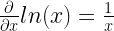
4: And, finally derivative of ln(x) is

Loss function is defined as

The logit function which feeds into the loss function is

And finally, z is a linear function of x values with  β coefficients which feeds in  the logit function

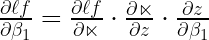
Now, we want to find the derivative or slope of loss function with respect to β coefficients i.e.

This equation can be expanded to individual components of loss function ( ), logit, and z

Let’s calculate the individual components of this formula. The first component is

The second component:

Since,

Finally, the third component

Hence, the product of three components will provide us with the derivative of the loss function with respect to the beta coefficients

Similarly,

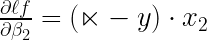
and,

That’s it.