In the last part of this series on fundamental machine learning, you learned about regularization and cross-validation. Here, you will gain a sound understanding of model hyper-parameter tuning to develop robust models. The machines do learn but they still need a good human tutor. In the last part, you were also introduced to my paternal grandmother to learn about regularization. This time let me introduce my maternal grandfather with a story. He and his radio will eventually help us understand the principles behind hyper-parameter tuning.

Color Pencils

My maternal grandfather was in the police which is considered as one of the more corrupt institutions in India. My cousin often tells this story. Our grandfather used to prepare certain monthly reports for his police station. This work required him to work with several color pencils. One day he was preparing these reports at home. My cousin saw him with all the pretty and colorful pencils. He asked grandpa to give him a few pencils. To his surprise, grandpa walked him to the neighborhood market a couple of miles from their house. After buying new pencils, when they were returning home my cousin asked, “Grandpa, we had so many similar pencils at home then why did you buy me new ones?“. Grandpa answered, “Those pencils at home belong to the Government of India. They are meant to be used for official work.”

Grandpa could have easily given a few of his official pencils to my cousin without anybody taking notice. Somehow, whenever my cousin tells this story both of us feel proud. Both of us, after all these years, are so glad that grandpa chose to walk those extra miles to the market.

I don’t have many memories of grandpa since he died when I was very young. I only remember an old radio that he used to own and I was completely fascinated with that radio.

Radio and Model Hyper-Parameter Tuning

It was a large wooden radio with a couple of round tuners. I used to love rotating those tuners to see the red dial move up and down. Other than giving kids something to play with, the purpose of those tuners was to connect the radio to the station. When the radio was not tuned it used to make funny noises. Once tuned, it played the melodious music which we all used to listen to while having our dinner.

The idea of machine learning hyper-parameter tuning is the same as using tuners for the radio. The effort is to identify the right setting for the model’s hyper-parameters to decipher music out of the seemingly noisy data. If you recall, we had two hyper-parameters, alpha (α) and lambda ( λ), in the elastic net model we trained in the last part. The loss function was:

Think of these hyper-parameters (α and λ) as the round tuners for the radio. The values of these hyper-parameters are changed slowly to decipher the signals hidden in the data. We will come back to the loss functions later in the article. The loss functions are kind of like FM and AM channels for the radio station. But before that let’s go back to the model we are working on throughout this series of articles.

Improving Models using Hyper-Parameter Tuning

Remember, we developed three different models in the last part using different variants of the loss function. The objective of all these models was to get the lowest value for the mean square error (MSE). The first term in the loss function (LF) was the MSE i.e . The second regularization term imposes constraints to avoid overfitting 

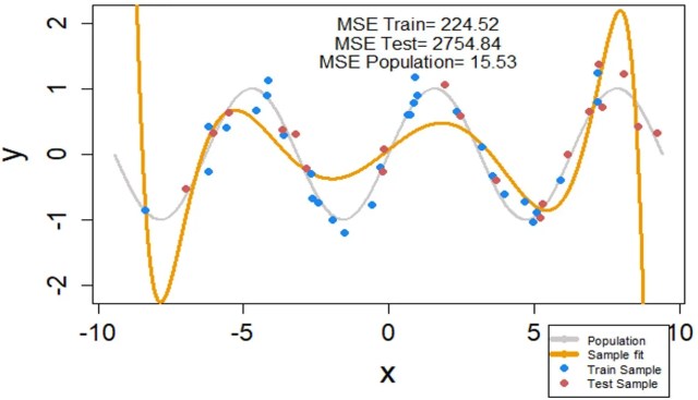
Let me quickly share the results of the final model we built at the end of the last article. Out of the three models, this model had the minimum MSE. Here, we kept the value of α constant at 1 – which is the Lasso regularization. We changed the value of λ. This change in λ was also hyper-parameter tuning.

Now that we have got some understanding of hyper-parameter tuning, let’s change both the hyper-parameters in the objective function simultaneously. The objective is still to get the minimum value for the MSE.

Hyper-Parameter Tunning – Changing both α and θ (Caret Package)

Caret Package in R offers the functionality to change these hyper-parameters simultaneously. You could find the entire code used for this series of articles at this link Regularization – Lasso & Ridge (Elastic Net) and Cross-Validation. Model-4 onwards in this code contains the analysis you will see in the subsequent segments.

When we perform a detained hyper-parameter tuning we are supposed to fit the underlying sine curve in the data to a greater extent. Let’s see the results. Firstly, there is a significant improvement in reduction of MSE values for both the training and test samples from the best fit we observed last time. For instance, the MSE for the test set has gone down from 2754.84 to 14.74 with the new values of hyper-parameters. How does the fit look?

Ouch! That was completely unexpected. The ripples for the expected sine curve have completely disappeared. With the best-tuned hyper-parameters, we have got an almost flat line bent at the corners. What is going on here?  To understand, let’s just fit a straight line to the training data points represented as the blue dots.

The MESs for both training and test samples have further reduced with the straight line. Eyes trained in statistics would identify the problem in a straight line fit to this data set through the analysis of error terms. You will soon realize, in this case, the MSE is not the only objective function one must look at.

Loss Functions – Not All Objectives are Same

A model can have other objectives than minimizing MSE. As mentioned earlier, these objectives are kind of like the AM and FM channels on the radio. This means sometimes you tune your radio for an AM channel (MSE) and other time for an FM (other objectives). In this case, we want to reduce the MSE (i.e. the overall error in estimation of Y using polynomials of X). Moreover, we also want the curve to fit the underlying sine curve.

As a solution, you could create your own customized loss function to achieve both these objectives. Then you can identify the optimal value for this new objective using the gradient descent approach. Another solution is to identify other metrics that could capture the degree of underlying fit to the data. Then, the two objectives values can be compared to identify the optimal values of hyper-parameters.

It turned out that for this problem the second objective could be satisfied with the R-Squared value. Then using Caret you could get different values of MSE and R-Squared values for different values of hyper-parameters. The lowest value of MSE along with the highest value of R-Squared will result in the satisfaction of both the objectives.  Let’s plot MSE and R-Squared to identify such condition. RMSE is the square root of MSE.

As you must have noticed, R-Squared value increases without much increase in the RMSE value as we move from left to right in the plot. If we settle for the minimum RMSE or MSE value, the R-Squared value is less than 0.3. However, if we let the RMSE increase by a few notches then the R-Squared rises to above 0.65. It turned out this happens for the following values of the hyper-parameters.

α = 1

λ = 0.00295

Final Model with Optimal Hyper-Parameters

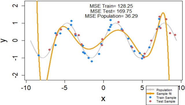
Let’s fit the data with these optimal values of hyper-parameters (α and λ). 

The MSE for both training and test set is much lower for this model than the one we observed last time. MSE of the test data has gone down from 2754 to 169. This is still higher than the straight line MSE of 0.43. What you have gained by losing the MSE is a relatively better fit for the data.

Sign-off Note

Tuning hyper-parameters requires a lot of thinking and requires a lot of supervision. The machines do learn but they still need a good human tutor.

See you all soon with an exciting series on deep learning and deep neural networks.