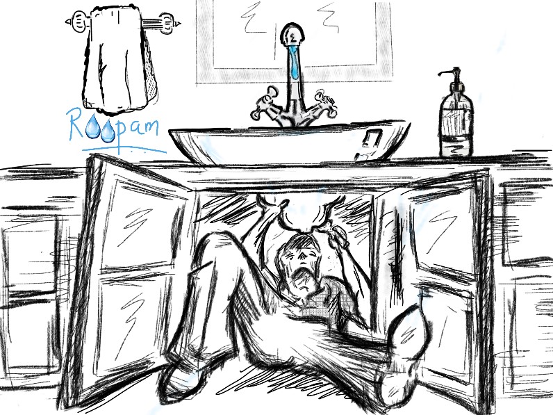
---

Welcome back to this series of articles on deep learning and neural networks. In the last part, you learned how training a deep learning network is similar to a plumbing job. This time you will learn the math of deep learning. We will continue to use the plumbing analogy to simplify the seemingly complicated math. I believe you will find this highly intuitive. Moreover, understanding this will provide you with a good idea about the inner workings of deep learning networks and artificial intelligence (AI) to build an AI of your own. We will use the math of deep learning to make an image recognition AI in the next part. But before that let’s create the links between…

The Math of Deep Learning and Plumbing

Last time we noticed that neural networks are like the networks of water pipes. The goal of neural networks is to identify the right settings for the knobs (6 in this schematic) to get the right output given the input.

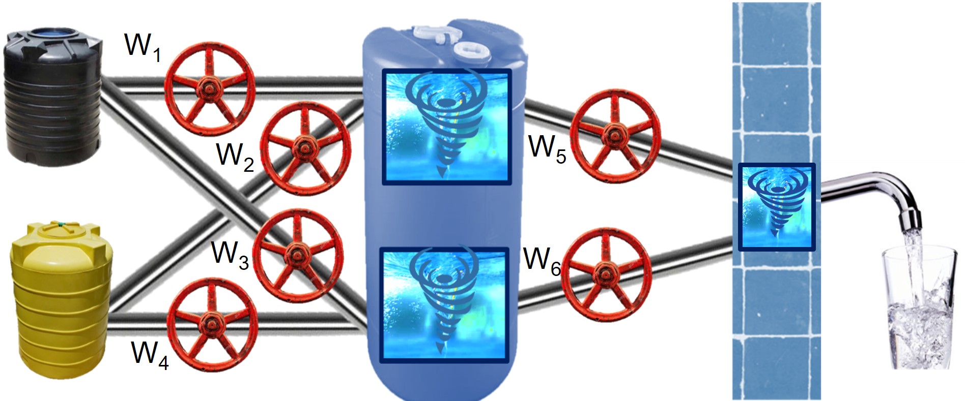
Shown below is a familiar schematic of neural networks almost identical to the water pipelines above. The only exception is the additional bias terms (b₁,b₂, and b₃) added to the nodes.

In this post, we will solve this network to understand the math of deep learning. Note that a deep learning model has multiple hidden layers, unlike this simple neural network. However, this simple neural network can easily be generalized to the deep learning models. The math of deep learning does not change a lot with additional complexity and hidden layers. Here, our objective is to identify the values of the parameters {W (W₁,…, W₆) and b (b₁,b₂, and b₃)}. We will soon use the backpropagation algorithm along with gradient descent optimization to solve this network and identify the optimal values of these weights.

Backpropagation and Gradient Descent

In the previous post, we discussed that the backpropagation algorithm works similar to me shouting back at my plumber while he was working in the duct. Remember, I was telling the plumber about the difference in actual water pressure from the expected. The plumber of neural networks, unlike my building’s plumber, learns from this information to optimize the positions of the knobs. The method that the neural networks plumber uses to iteratively correct the weights or settings of the knobs is called gradient descent.

We have discussed the gradient descent algorithm in an earlier post to solve a logistic regression model. I recommend that you read that article to get a good grasp of the things we will discuss in this post. Essentially, the idea is to iteratively correct the value of the weights (W_i) to produce the least difference between the actual and the expected values of the output. This difference is measured mathematically by the loss function i.e . The weights (W_i and b_i) are then iteratively improved using the gradient of the loss function wrt weights using this expression:

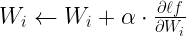
Here, α is called the learning rate – it’s a hyperparameter and stays constant. Hence, the overall problem boils down to the identification of partial derivatives of the loss function with respect to the weights i.e. . For our problem, we just need to solve the partial derivatives for W₅ and W₁. The partial derivatives for other weights can then be easily derived using the same method used for W₅ and W₁.

Before we solve these partial derivatives, let’s do some more plumbing jobs and look at a tap to develop intuitions about the results we will get from the gradient descent optimization.

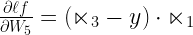
Intuitive Math of Deep Learning for W₅ & A Tap

We will use this simple tap to identify an optimal setting for its knob. In this process, we will develop intuitions about gradient descent and the math of deep learning. Here, the input is the water coming from the pipe on the left of the image. Moreover, the output is the water coming out of the tap. You use the knob, on the top of the tap, to regulate the quantity of the output water given the input. Remember, you want to turn the knob in such a way that you get the desired output (i.e the quantity of water) to wash your hands. Keep in mind, the position of the knob is similar to the weight of a neural networks’ parameters. Moreover, the input/output water is similar to the input/output variables.

Essentially, in math terms, you are trying to identify how the position of the knob influences the output water. The mathematical equation for the same is:

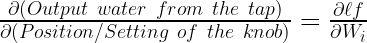
If you understand the influence of the knob on the output flow of water you can easily turn it to get the desired output. Now, let’s develop an intuition about how much to twist the knob. When you use a tap you twist the knob until you get the right flow or the output. When the difference between the desired output and the actual output is large then you need a lot of twisting. On the other hand, when the difference is less then you turn the knob gently.

Moreover, the other factor on which your decision depends on is the input from the left pipe. If there is no water flowing from the left pipe then no matter how much you twist the knob it won’t help. Essentially, your action depends on these two factors.

Your decision to turn the knob depends on
Factor 1: Difference between the actual output and the desired Output and
Factor 2: Input from the grey pipe on the left

Soon you will get the same result by doing a seemingly complicated math for the gradient descent to solve the neural network.

For our network, the output difference is and input is . Hence,

Disclaimer

Please note, to make the concepts easy for you to understand, I had taken a few liberties while defining the factors in the previous section. I will make these factors much more theoretically grounded at the end of this article when I will discuss the chain rule to solve derivatives. For now, I will continue to take more liberties in the next section when I discuss the other weight modification for other parameters of neural networks.

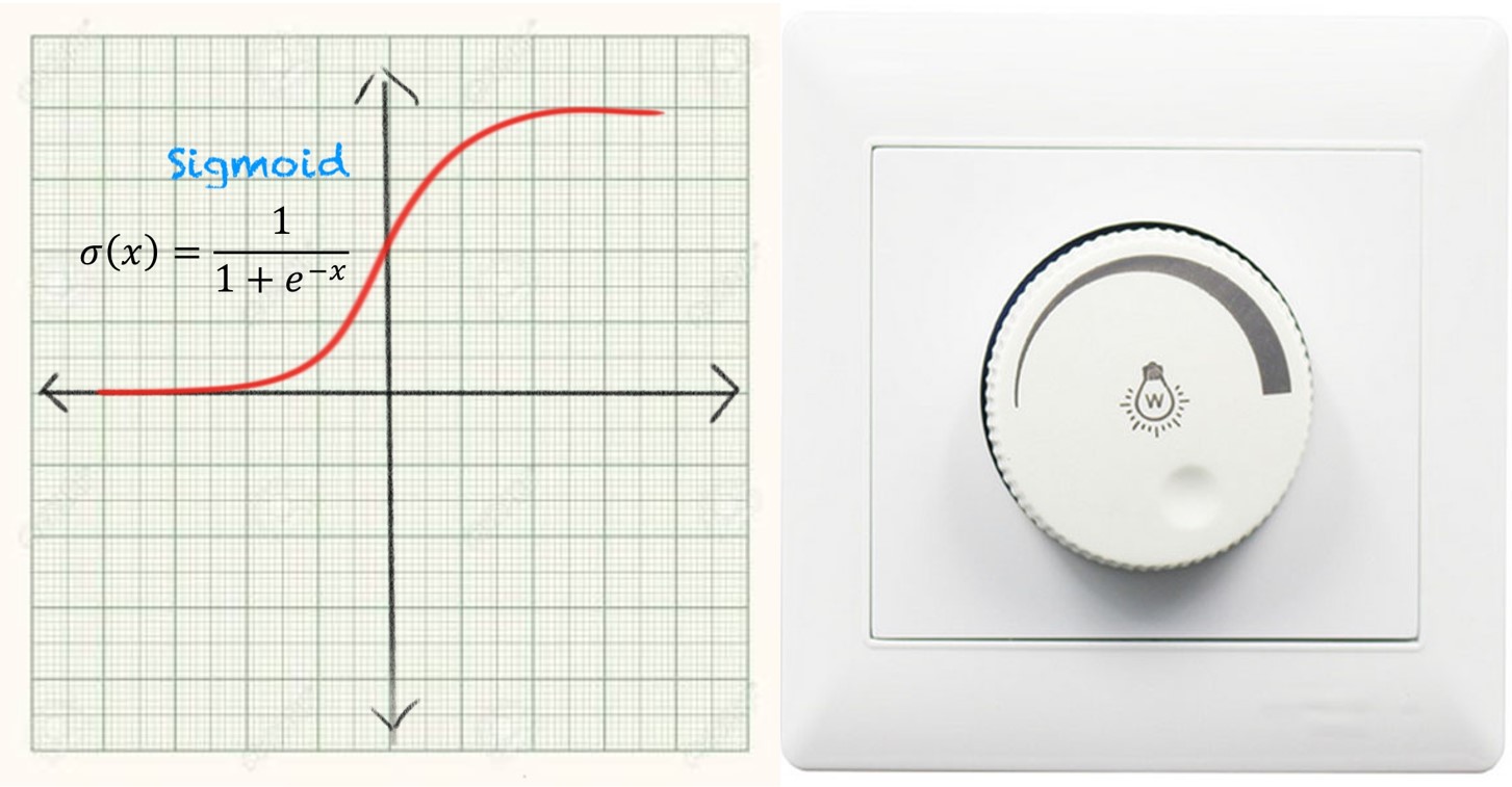
Add More Knobs to Solve W₁ – Intuitive Math of Deep Learning

Neural networks, as discussed earlier, have several parameters (Ws and bs). To develop an intuition about the math to estimate the other parameters further away from the output (i.e. W₁), let’s add another knob to the tap.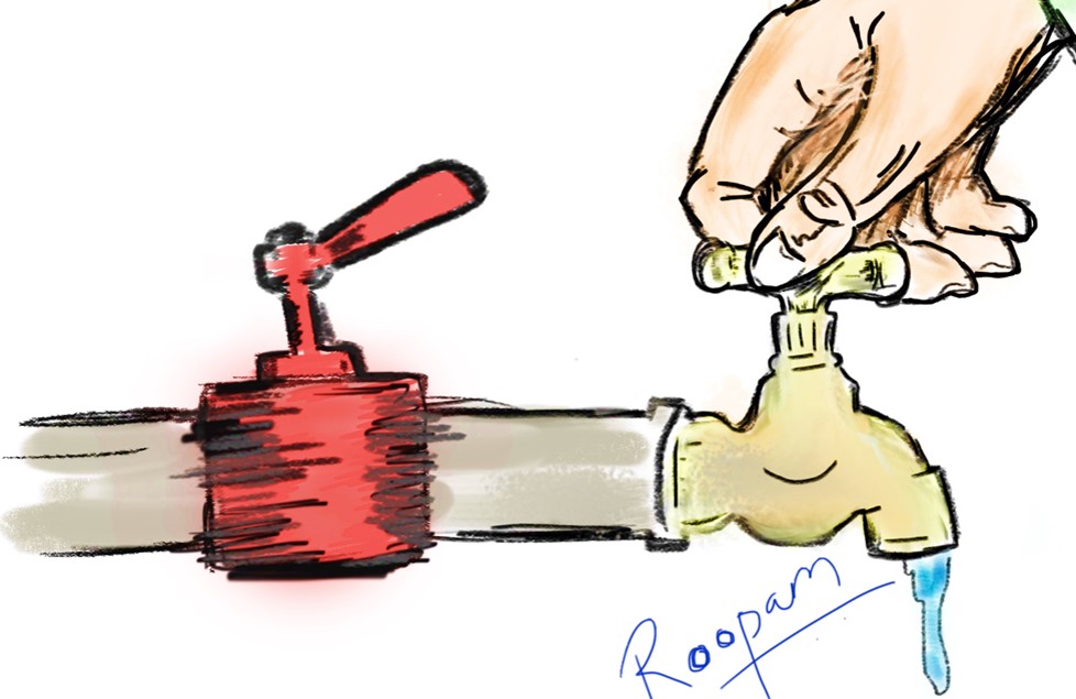 
Here, we have added a red regulator knob to the tap we saw in the earlier section. Now, the output from the tap is governed by both these knobs. Referring to the neural network’s image shown earlier, the red knob is similar to the parameters (W₁, W_2, W₃, W_4, b_1, and b₂) added to the hidden layers. The knob on top of the brass tap is like the parameters to the output layer (i.e. W₅, W₆, and b₃).

Now, you are also using the red knob, in addition to the knob on the tap, to get the desired output from the tap. Your effort of the red knob will depend on these factors.

Your decision to turn the red knob depends on
Factor 1: Difference between the actual and the desired final output and
Factor 2: Position / setting of the knob on the brass tap and
Factor 3: Change in input to the brass tap caused by the red knob and
Factor 4: Input from the pipe on the left into the red knob

Here, as already discussed earlier, factor 1 is . W₅ is the setting/weight for the knob of the brass tap. Factor 3 is . Finally, the last factor is the input or X₁. This completes our equation as:

Now, before we do the math to get these results, we just need to discuss the components of our neural network in mathematical terms. We already know how it relates to the water pipelines discussed earlier.

Let’s start with the nodes or the orange circles in the network diagram.

Nodes of Neural Networks

Here, these two networks are equivalent except the additional b₁ or bias for the neural networks.

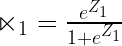
The node for the neural network has two components i.e. sum and non-linear. The sum component (Z₁) is just a linear combination of the input and the weights.

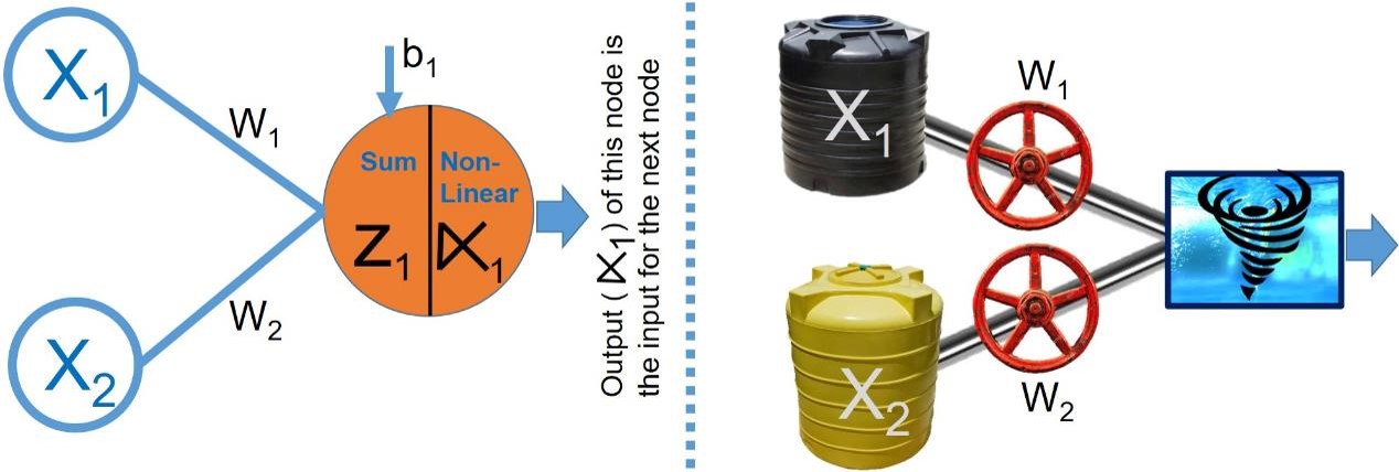
The next term, i.e. non-linear, is the non-linear sigmoid activation function (). As discussed earlier, it is like a regulator of a fan that keeps the value of   between 0 and 1 or on/off.

The mathematical expression for this sigmoid activation function () is:

The nodes in both the hidden and output layer behave the same as described above. Now, the last thing is to define the loss function () which is to measure the difference between the expected and actual output. We will define the loss function for most common business problems.

Classification Problem – Math of Deep Learning

In practice, most business problems are about classification. They have binary or categorical outputs/answers such as:

• Is the last credit card transaction fraudulent or not?
• Will the borrower return the money or not?
• Was the last email in your mailbox a spam or ham?
• Is that a picture of a dog or cat? (this is not a business problem but a famous problem for deep learning)
• Is there an object in front of an autonomous car to generate a signal to push the break?
• Will the person surfing the web respond to the ad of a luxury condo?

Hence, we will design the loss function of our neural network for similar binary outputs. This binary loss function, aka binary cross entropy, can easily be extended for multiclass problems with minor modifications.

Loss Function and Cross Entropy

The loss function for binary output problems is:

This expression is also referred to as binary cross entropy. We can easily extend this binary cross-entropy to multi-class entropy if the output has many classes such as images of dog, cat, bus, car etc. We will learn about multiclass cross entropy and softmax function in the next part of this series. Now that we have identified all the components of the neural network, we are ready to solve it using the chain rule of differential equations.

Chain Rule for W₅ – Math of Deep Learning

We discussed the outcome for change observed in the loss function() wrt to change in W₅ earlier using a single knob analogy. We know the answer to  is equal to  . Now, let’s derive the same thing using the chain rule of derivatives. Essentially, this is similar to the change in water pressure observed at the output by turning the knob on the top of the tap. The chain rule states this:

The above equation for chain rule is fairly simple since equation on the right-hand side will become the one on the left-hand side by simple division. More importantly, these equations suggest that the change in the output essentially the change observed at different components of the pipeline because of turning the knob.

Moreover, we already discussed the loss function which is the binary cross entropy i.e.

The first component of the chain rule is  which is

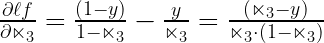
This was fairly easy to compute if you only know that derivative of a natural log function is

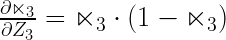
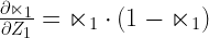
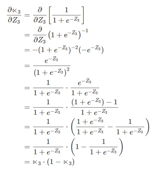
This second component of the step function is . This derivative of the sigmoid function ( ) is slightly more complicated.  You could find here a detailed solution to the derivative of the sigmoid function. This implies,

Finally, the third component of chain rule is again very easy to compute i.e.

Since we know,

Now, we just multiply these three components of the chain rule and we get the output i.e.

Chain Rule for W₁ – Math of Deep Learning

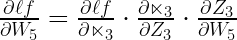
The chain rule for the red knob or the additional layer is just an extension of the chain rule of the knob on the top of the tap. This one has a few more components because the water has to travel through more components i.e.

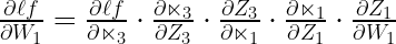
The first two components are exactly the same as the knob of the tap i.e. W₅. This makes sense since the water is flowing through the same pipeline towards the end. Hence, we will calculate the third component

The fourth component is the derivative of the sigmoid function i.e. the derivative of the sigmoid function

The fifth and the final component is again easy to calculate.

That’s it. We now multiply these five components to get the results we have already seen for the additional red knob.

Sign-off Node

This part of the series became a little math heavy. All this, however, will help us a lot when we  will build an artificial intelligence to recognize images. See you then.