This article is a continuation of our manufacturing case study example to forecast tractor sales through time series and ARIMA models. You can find the previous parts at the following links:
Part 3: Introduction to ARIMA models for forecasting
In this part, we will use plots and graphs to forecast tractor sales for PowerHorse tractors through ARIMA. We will use ARIMA modeling concepts learned in the previous article for our case study example. But before we start our analysis, let’s have a quick discussion on forecasting:
Trouble with Nostradamus

Human Obsession with Future & ARIMA – by Roopam
Humans are obsessed about their future – so much so that they worry more about their future than enjoying the present. This is precisely the reason why horoscopists, soothsayers, and fortune tellers are always in high-demand. Michel de Nostredame (a.k.a Nostradamus) was a French soothsayer who lived in the 16th century. In his book Les Propheties (The Prophecies) he made predictions about important events to follow till the end of time. Nostradamus’ followers believe that his predictions are irrevocably accurate about major events including the World Wars and the end of the world. For instance in one of the prophecies in his book, which later became one of his most debated and popular prophesies, he wrote the following
“Beasts ferocious with hunger will cross the rivers
The greater part of the battlefield will be against Hister.
Into a cage of iron will the great one be drawn,
When the child of Germany observes nothing.”
His followers claim that Hister is an allusion to Adolf Hitler where Nostradamus misspelled Hitler’s name. One of the conspicuous thing about Nostradamus’ prophecies is that he never tagged these events to any date or time period. Detractors of Nostradamus believe that his book is full of cryptic pros (like the one above) and his followers try to force fit events to his writing. To dissuade detractors, one of his avid followers (based on his writing) predicted the month and the year for the end of the world as July 1999 – quite dramatic, isn’t it? Ok so of course nothing earth-shattering happened in that month of 1999 otherwise you would not be reading this article. However, Nostradamus will continue to be a topic of discussion because of the eternal human obsession to predict the future.
Time series modelling and ARIMA forecasting are scientific ways to predict the future. However, you must keep in mind that these scientific techniques are also not immune to force fitting and human biases. On this note let us return to our manufacturing case study example.
ARIMA Model – Manufacturing Case Study Example
Back to our manufacturing case study example where you are helping PowerHorse Tractors with sales forecasting for them to manage their inventories and suppliers. The following sections in this article represent your analysis in the form of a graphic guide.
| You could find the data shared by PowerHorse’s MIS team at the following link Tractor Sales. You may want to analyze this data to revalidate the analysis you will carry-out in the following sections. |
Now you are ready to start with your analysis to forecast tractors sales for the next 3 years.
Step 1: Plot tractor sales data as time series
To begin with you have prepared a time series plot for the data. The following is the R code you have used to read the data in R and plot a time series chart.
data = read.csv('http://ucanalytics.com/blogs/wp-content/uploads/2015/06/Tractor-Sales.csv')
data = ts(data[,2],start = c(2003,1),frequency = 12)
plot(data, xlab='Years', ylab = 'Tractor Sales')
Clearly the above chart has an upward trend for tractors sales and there is also a seasonal component that we have already analyzed an earlier article on time series decomposition.
Step 2: Difference data to make data stationary on mean (remove trend)
The next thing to do is to make the series stationary as learned in the previous article. This to remove the upward trend through 1st order differencing the series using the following formula:
| 1st Differencing (d=1) |  |
The R code and output for plotting the differenced series are displayed below:
plot(diff(data),ylab='Differenced Tractor Sales')
Okay so the above series is not stationary on variance i.e. variation in the plot is increasing as we move towards the right of the chart. We need to make the series stationary on variance to produce reliable forecasts through ARIMA models.
Step 3: log transform data to make data stationary on variance
One of the best ways to make a series stationary on variance is through transforming the original series through log transform. We will go back to our original tractor sales series and log transform it to make it stationary on variance. The following equation represents the process of log transformation mathematically:
| Log of sales |  |
The following is the R code for the same with the output plot. Notice, this series is not stationary on mean since we are using the original data without differencing.
plot(log10(data),ylab='Log (Tractor Sales)')
Now the series looks stationary on variance.
Step 4: Difference log transform data to make data stationary on both mean and variance
Let us look at the differenced plot for log transformed series to reconfirm if the series is actually stationary on both mean and variance.
| 1st Differencing (d=1) of log of sales |  |
The following is the R code to plot the above mathematical equation.
plot(diff(log10(data)),ylab='Differenced Log (Tractor Sales)')
Yes, now this series looks stationary on both mean and variance. This also gives us the clue that I or integrated part of our ARIMA model will be equal to 1 as 1st difference is making the series stationary.
Step 5: Plot ACF and PACF to identify potential AR and MA model
Now, let us create autocorrelation factor (ACF) and partial autocorrelation factor (PACF) plots to identify patterns in the above data which is stationary on both mean and variance. The idea is to identify presence of AR and MA components in the residuals. The following is the R code to produce ACF and PACF plots.
par(mfrow = c(1,2))
acf(ts(diff(log10(data))),main='ACF Tractor Sales')
pacf(ts(diff(log10(data))),main='PACF Tractor Sales')

Since, there are enough spikes in the plots outside the insignificant zone (dotted horizontal lines) we can conclude that the residuals are not random. This implies that there is juice or information available in residuals to be extracted by AR and MA models. Also, there is a seasonal component available in the residuals at the lag 12 (represented by spikes at lag 12). This makes sense since we are analyzing monthly data that tends to have seasonality of 12 months because of patterns in tractor sales.
Step 6: Identification of best fit ARIMA model
Auto arima function in forecast package in R helps us identify the best fit ARIMA model on the fly. The following is the code for the same. Please install the required ‘forecast’ package in R before executing this code.
require(forecast)
ARIMAfit = auto.arima(log10(data), approximation=FALSE,trace=FALSE)
summary(ARIMAfit)
| Time series: | log10(Tractor Sales) | |
| Best fit Model: ARIMA(0,1,1)(0,1,1)[12] | ||
| ma1 | sma1 | |
| Coefficients: | -0.4047 | -0.5529 |
| s.e. | 0.0885 | 0.0734 |
| log likelihood=354.4 | ||
| AIC=-702.79 | AICc=-702.6 | BIC=-694.17 |
The best fit model is selected based on Akaike Information Criterion (AIC) , and Bayesian Information Criterion (BIC) values. The idea is to choose a model with minimum AIC and BIC values. We will explore more about AIC and BIC in the next article. The values of AIC and BIC for our best fit model developed in R are displayed at the bottom of the following results:
As expected, our model has I (or integrated) component equal to 1. This represents differencing of order 1. There is additional differencing of lag 12 in the above best fit model. Moreover, the best fit model has MA value of order 1. Also, there is seasonal MA with lag 12 of order 1.
Step 6: Forecast sales using the best fit ARIMA model
The next step is to predict tractor sales for next 3 years i.e. for 2015, 2016, and 2017 through the above model. The following R code does this job for us.
par(mfrow = c(1,1))
pred = predict(ARIMAfit, n.ahead = 36)
pred
plot(data,type='l',xlim=c(2004,2018),ylim=c(1,1600),xlab = 'Year',ylab = 'Tractor Sales')
lines(10^(pred$pred),col='blue')
lines(10^(pred$pred+2*pred$se),col='orange')
lines(10^(pred$pred-2*pred$se),col='orange')
The following is the output with forecasted values of tractor sales in blue. Also, the range of expected error (i.e. 2 times standard deviation) is displayed with orange lines on either side of predicted blue line.

Now, forecasts for a long period of 3 years is an ambitious task. The major assumption here is that the underlining patterns in the time series will continue to stay the same as predicted in the model. A short-term forecasting model, say a couple of business quarters or a year, is usually a good idea to forecast with reasonable accuracy. A long-term model like the one above needs to evaluated on a regular interval of time (say 6 months). The idea is to incorporate the new information available with the passage of time in the model.
Step 7: Plot ACF and PACF for residuals of ARIMA model to ensure no more information is left for extraction
Finally, let’s create an ACF and PACF plot of the residuals of our best fit ARIMA model i.e. ARIMA(0,1,1)(0,1,1)[12]. The following is the R code for the same.
par(mfrow=c(1,2))
acf(ts(ARIMAfit$residuals),main='ACF Residual')
pacf(ts(ARIMAfit$residuals),main='PACF Residual')
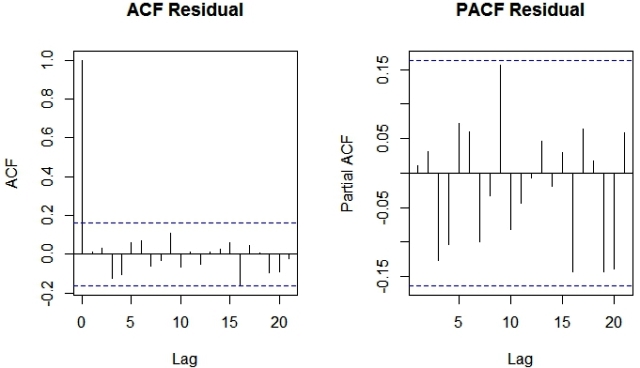
Since there are no spikes outside the insignificant zone for both ACF and PACF plots we can conclude that residuals are random with no information or juice in them. Hence our ARIMA model is working fine.
However, I must warn you before concluding this article that randomness is a funny thing and can be extremely confusing. We will discover this aspect about randomness and patterns in the epilogue of this forecasting case study example.
Sign-off Note
I must say Nostradamus was extremely clever since he had not tagged his prophecies to any time period. So he left the world with a book containing some cryptic sets of words to be analysed by the human imagination. This is where randomness becomes interesting. A prophesy written in cryptic words without a defined time-period is almost 100% likely to come true since humans are the perfect machine to make patterns out of randomness.
Let me put my own prophesy for a major event in the future. If someone will track this for the next 1000 years I am sure this will make me go in the books next to Nostradamus.
A boy of strength will rise from the home of the poorWill rule the world and have both strong friends and enemiesHis presence will divide the world into halfThe man of God will be the key figure in resolution of this conflict
Hi Roopam,
Great article, very good explanation. Thank you.
Here is a suggestion to help the readers:.
As the data is not in a time-series format, it will help if we convert it to a time-series when plotting it.
Change the code in the following steps:
Step 1: plot(ts(data[,2]), xlab=”Years”, ylab = “Tractor Sales”)
Step 2: plot(diff(ts(data[,2])), xlab=”Years”, ylab = “Diff Tractor Sales”)
Step 3: plot(log(ts(data[,2])), xlab=”Years”, ylab = “Log Tractor Sales”)
Keep up the great work.
Regards
Ram
Thanks Ram for sharing your code to convert data into time series data format. I did miss out on this, now have included an extra step in the beginning for the same. Appreciate you help!
Cheers
Roopam
Cool, Thank you bro.
hello ram,
Thanks for sharing valuable information..could you please suggest me the best material for understanding forecasting inventory using ARIMA in depth??I couldn’t understand the types of models exists in ARIMA..
hello im doing my thesis using arima(autoregressive integrated moving average ) modelling techniqe but i dont know what should i do to study the arima . as it needed a practicle study bt i just read it as theoraticle . please guide me in this case i’ll be gratefull to u !!!!
Play around with your data – plot them and make naive predictions in the beginning and then figure out how to improve those predictions using other techniques (like ARIMA, neural networks etc.). I think that’s the best way to practice and get a practical exposure – play with your data. All the best.
Roopam,
you have already converted into time series in your first step:
data<-read.csv(“[location of data]“)
data<-ts(data[,2],start = c(2003,1),frequency = 12)
plot(data, xlab=”Years”, ylab = “Tractor Sales”)
Then why this correction.Pls update.
Rgrds,
Saurabh Gupta
thank you for your help
Sarabh: you are right. I think I missed to paste this step in the original post and hence took Ram’s suggestion. Anyway this doesn’t change the results.
Newton: sorry missed your earlier comment, but to add, data[,2] piece in the code is to make R realise that the time series is in the 2nd column of the dataset.
Roopam,
1:I have 2 years day wise data of stock price.what frequency I should take in this case for next 1 year day wise prediction.
2 :I have one day minute wise data .what frequency I should take for next day forecast minute wise?
Actually I want to know what is frequency wrt timeseries and prediction?
Please I need a guide on how to run ARIMA using R, help me with some materials that is well explanatory. Thanks
So what you’re saying at the end is that, by attempting to shoehorn all of history into Nostradamus’s predictions, people are overfitting the data but don’t realize it because they’re watching the training set error (i.e. performance on events that have already happened) rather than the generalization error 🙂
Hindsight is always 20/20 🙂
This data looks a lot like the world famous Box-Jenkins International Airline Passenger series example. It has the same length of the data too. When I compare the two time series and I divide the one column by the other for each data point and plot the ratio it screams out that I am right. Even the LOG transform is right from the Box-Jenkins text book(which is unneeded and actually harmful as the use of LOGS was incorrect as the outliers in the data creates a false positive on the F test suggesting that LOGS are useful).
You got it right Tom, it is a version of the famous Airline data. I used this data, instead of a simulated data, as a tribute to the pioneers of ARIMA: George Box and Gwilym Jenkins. Thanks for pointing this out – I was sure someone will crack this riddle 🙂 .
However, I am curious to investigate your statement on the log transformation of this data. Please provide some more details.
Cheers
Roopam
Roopam,
Box and Jenkins didn’t have the tools and knowledge that we do today. They had slow computers and no ability to search for outliers like now. If you ignore outliers, you will have a false conclusion that you need logs. However, if you look for outliers and build dummy variables for them (ie stepup regression with deterministic 0/1 dummy variables) then you will not use logs and NOT have a forecast that goes as high (incorrectly) as there’s did. We have a presentation on our website that discusses that I presented at the IBF in 2009 on this here. http://www.autobox.com/cms/index.php/news/54-data-cleansing-and-automatic-procedures
Hello Roopam
First of all, congratulations, I have read your case study example and it is very clear. But I have a question, in your first part you said: “Eventually, you will develop an ARIMA model to forecast sale / demand for next year. Additionally, you will also investigate the impact of marketing program on sales by using an exogenous variable ARIMA model.” I don´t know if part 4 is final part or I have to wait until a future delievery to read about how we can used a exogenous variable like “marketing program. I hope you’re soon to continue with your example , because frankly I’m desperate to know how this story ends.
Thanks
Gabriel Cornejo
CHILE
Thanks Gabriel and yes there is a final part left in this case study with an exogenous variable i.e. marketing expense. Hope you will enjoy that as well.
Great Article with live examples..
Thanks a lot Roopam 🙂
Great article! I appreciate it but how can we get the actual predicted value and the R-code that is used to plot the actual values and the predicted values for the differenced and log transformed data?
Thanks Demiss. If I am getting you question right, you will find the piece of code in the step 6 in this article.
Thanks for Roopam for your prompt response! It is not still clear for me and the code in step 6 doesnt give me what I wanted. I am thinking the actual predicted value is the summation of the forecasted data plus the trend value (if there is trend) in the differenced time series stationary data. I will be happy if you clarify for me how can we get the actual predicted(forecasted )value. thanks!
Ok, got you. Our final model was built with log10(Tractor Sales) data i.e we had log-transformed our original tractor sales data. The remaining operations i.e. differencing and moving average are in-built in our Arima model i.e. Best fit Model: ARIMA(0,1,1)(0,1,1)[12] (see step 5).
Trend and other variations are part of this ARIMA model except log transformation. Hence for making the final forecast we just need to exponentially-transform the data by raising it to the power 10. That is exactly what I did to arrive at the final values in the step 6. I did the same for margin of errors.
Thanks again for your reply and explanation. If you don’t get the best model using the already in-built model, how can we proceed to get the actual predicted value? My model is based on differencing and AIC information criteria. If you can give me your e-mail address, I can send the details since I got a wrong model with high AIC value using the in-built ARIMA model.
Any way, thank you for your explanation and prompt response but my model is a bit far than what you have done.
Dear Roopam
Thanks for the useful article,
i have a question ;Isn’t it neccessary to check the stationary by the coomon tests and ADF? It seems that we use log transformatio to remove the non-stationary in the variance and then take difference to remove the non-stationary in the mean, but before doing that neither outlier test nor stationary test had been done!
Thanks Mahdi, there are unit root tests to check stationarity such as ADF. These tests are really convenient however I personally prefer simple visualisation over statistical tests and p-values. In case there is confusion use these tests in addition to visualisation. In the same spirit, I prefer histograms or scatter plots any day over the values of mean, standard deviation, and correlation coefficient. I guess every analyst has their preferred style and mine is certainly data visualisation.
Dear Roopam
thanks for the explanation, i want to know if you have got other article talking about central and disperse indices like mean,std,c.v., … and also VAR(value at risk) as clear as the article above with data available?
Dear Mahdi,
I am yet to write detailed articles on these topics. However, I believe You might find the following articles useful:
Article 1
Article 2
Article 3
Cheers
Hi Roopam,
I’m a novice in this field and I’m still struggling to figure out how the predicted value from the arima model is obtained. In other words, if I have to manually calculate the one-step ahead predicted value after fitting the model, what is the formula to be used?
Hoping you’ll be able to clear my confusion.
(Sorry if my question is too basic)
Sanya: in the simplest form, think of ARIMA model like the following equation (simple regression model):
Sales(Future) = Sales(Past) + 300 + Random Variable (Ignore random variable for now)
Now, if Sales(Past) = 1000 units you could easily calculate Sales(Future) = 1300 units.This is a simple ARIMA model with just an Integrated term i.e. ARIMA(0,1,0).
The above model could be extended to include more terms like Auto-Regressive and Moving-Average parts. At the end, you will get an equation similar to our simple model above. Once you will substitute the right values in the past you will arrive at the value for future.
I want help on how to use Neural network and SVM model for time series forecasting as you have given using ARIMA step by step
Will write about usage of Neural Nets for forecasting in some article soon. SVM is not used for time series forecasting.
Hi Roopam,
Nice article.But I have one doubt.How you check the series in not stationary over variance?
Thanks,
Smita
Smita, that’s a great question. I know you have addressed Roopam, but if I may, I would like to attempt to answer your concerns. A major caveat to ARIMA modeling is non-constant variance (non-stationary), but, when identified correctly, it can be a great resource to the time series modeler.
There are three ways (and reasons) to check your time series for changes in error variance.
1) The variance of the errors is changing by a discernible magnitude. For example, if you are looking at your series for changes in variance, it could be useful to test the relationship of the variance or standard deviation to the expected value, and if they are reasonably proportional, then a transformation could be in order. Potentially, you could have any number of possible Box-Cox transformations that could help stabilize the variance. Take a close look at the picture in the post I have linked below.
Source:http://stats.stackexchange.com/questions/18844/when-and-why-to-take-the-log-of-a-distribution-of-numbers
2) The variance of the errors is changing by a deterministic structure at a particular point in time. This is not to be confused with power transforms mentioned. The nature of these deterministic structures speaks more to a paradigm shift in variance rather than a continuous proportion. For example, if one were to split a data set in half, where the first half of the series has a variance of S, and the second half of the series has a variance of S*, we would need to be sure that the variances were not significantly different from another to justify changing the overall model. ARIMA models use an equal weighting scheme (OLS) unless specified otherwise — this is one of those times where this premise can hurt you. Switching over to a Generalized Linear Model, or Generalized Least Squares, within the framework of ARIMA estimation, allows us to account for non-constant error variance. By doing this, we can put “weights” on the data to dampen the impact of the increased variance. From there, we can normalize the data to better detect other useful changes in the data.
Source: http://www.unc.edu/~jbhill/tsay.pdf
3) Variance of the errors is itself a random variable subject to some ARIMA structure. If we have a structure in the variance of the errors that is representative of some repetitive pattern, then perhaps using a GARCH or ARCH model could help us. Notice how this is similar to the deterministic “paradigm shift” mentioned above. Imagine that error variance is subject to the same type of analysis that your typical ARIMA model is. There can be lags, leads, and changes in variance structure the can be identified as a function of time.
Of course, none of the above say much about the presence of outliers in your data; which, untreated, have the ability to suggest any of the above 3 cases when they would otherwise be unnecessary.. In fact, testing for outliers should preclude your analysis of change in variance. To tie off this response, a good visualization of the importance of outlier detection (and how the lack thereof can lead you astray) read this document starting on page 14. Link: http://www.autobox.com/pdfs/vegas_ibf_09a.pdf
Hii roopam, nice explanation about ARIMA.I learned ARIMA model from your website and now trying to apply it to forecast sales for stores. I have time series data with daily observation. So my first question what should be value of frequency for daily data in step 1 and when I followed above steps for my data series I am not getting reasonable forecast.Below is link to my data and code.Please help me asap.
Link to dataset: https://drive.google.com/file/d/0B-KJYBgmb044QlNUS3FhVFhUbE0/view?usp=sharing
This is my code:
data<-read.csv("Book5.csv")
View(data)
mydata<- ts(data[,2], start=1, end=181, frequency = 7)
View(mydata)
plot(mydata, xlab="Day", ylab = "Sales")
plot(diff(mydata),xlab="Day",ylab="Differenced Sales")
plot(log10(mydata),ylab="Log(Sales)")
plot(diff(log10(mydata)),ylab="Differenced Log (Sales)")
par(mfrow = c(1,2))
acf(ts(diff(log10(mydata))),main="ACF Sales", na.action = na.pass)
pacf(ts(diff(log10(mydata))),main="PACF Sales",na.action = na.pass)
require(forecast)
ARIMAfit <- auto.arima(log10(mydata))
summary(ARIMAfit)
pred <- predict(ARIMAfit, n.ahead= 181)
pred
class(pred$pred)
10^(pred$pred)
# Write CSV in R
write.csv(10^(pred$pred), file = "MyData.csv")
plot(mydata,type="l",xlim=c(1,181),ylim=c(1,6000),xlab = "Day",ylab = "Sales")
lines(10^(pred$pred),col="blue")
lines(10^(pred$pred+2*pred$se),col="orange")
lines(10^(pred$pred-2*pred$se),col="orange")
Your data has quite a few zeros for sales, I believe for days when the store is closed i.e. holidays. These holidays are also not completely regular (mostly on Sundays but there are several anomalies). However these holidays are pre-decided on the calendar. You may want to add an exogenous dummy variable for holidays i.e. working day =0 otherwise 1. Use xreg operator as described in this post. This will take care of this irregularity. Check how your model performs after this tweak.
Good one.
I was also going to suggest Patrick to use the xreg parameter.
For his data, it will be an array of length 181, containing 0’s and 1’s. ( Mostly 0’s and a few 1’s for holidays)
Note: If you use xreg in ARIMA, you have to use xreg in forecast as well.
I also noticed that the data is stationary. Hence the lag and log transformations are not required. Roopam, could you confirm?
Correction:
In my previous comment, I meant to say diff and not lag :
I also noticed that the data is stationary. Hence the diff and log transformations are not required. Roopam, could you confirm?
I am not sure about how to use xreg parameter. Can you please tell me what will be its value. Is it name of column which is having irregular 0’s. I did as follows:
require(forecast)
ARIMAfit <- auto.arima(log10(mydata),xreg= data$Sales, approximation=FALSE,trace=FALSE)
summary(ARIMAfit)
but it gives error like:
Error in model.frame.default(formula = x ~ xreg, drop.unused.levels = TRUE) :
variable lengths differ (found for 'xreg')
In addition: Warning message:
In !is.na(x) & !is.na(rowSums(xreg)) :
longer object length is not a multiple of shorter object length
Here is one way to proceed:
myts <- ts(data[,2], start=c(2013,1),frequency = 365)
print(myts)
# Create an array of holidays, using the counts. This will be used as xreg.
holiday = data[,2] == 0;
print(holiday)
require(forecast)
#Fit the model using holiday as xreg
ARIMAfit <- auto.arima(myts, approximation=FALSE,trace=FALSE, xreg=holiday);
summary(ARIMAfit)
#Define xreg for 2 weeks forecast, assuming that Sundays are holidays;
holiday=rep(c(rep(FALSE,6),T),2);
print(holiday)
# Forecast using xreg.
# Note: When you use xreg, the parameter n.ahead is not required.
fcast <- forecast(ARIMAfit, xreg=holiday)
print(fcast)
plot(fcast)
## End
Thanks Ram for help! The forecast using xreg are better but not close to actual values. Can you please suggest me something that I can do to forecast as close as possible values.I tried model with different frequency like 7,12,365.
Also I would like to tell you that I want to forecast only for two months august & september so used only past dataset of aug & september and it is giving some reasonable plots but not accurate.So what should I do to get more accurate forecast.Thanks in advance 🙂
This is plot of current forecast values:https://drive.google.com/file/d/0B-KJYBgmb044YlVDand1UmNnVTA/view?usp=sharing
Nice
Hi Patrick,
I agree, the forecast gives negative Sales for holidays. I am not sure how we can get a better forecast. I am sure Roopam will be able to provide help.
Here is one option you can try:
Create a new series excluding the 0 Sales. Then fit a model and do a forecast on this new series without xreg.
data.m = subset(data, Sales>0) ## Select non-zero sales
myts = ts(data.m[,2]) ## Do not specify the frequency for the series.
ARIMAfit = auto.arima(myts, approximation=FALSE,trace=FALSE) ## Do not use xreg
#Forecast for 2 months, assuming 52 business days. (No forecast for holidays)
fcast = forecast(ARIMAfit, h=52)
print(fcast)
plot(fcast)
## End
##Note: I have not done any transformation (diff or log) to the data, because the series is already stationary. (It has no trend, and has uniform variance).
@Patrick: I would recommend you to ask these questions:
1) Do you need a daily forecast? If yes, why?
A forecast of shorter duration tends to have a larger noise. In this case since from the logical point of view there is no obligation on shoppers to shop on Mondays instead of Tuesdays. This variation will influence the overall accuracy of your model. You may want to create a weekly forecast. This will take care of weekly holidays. Also, add a dummy trigger if there are additional holidays in that week. Moreover, you could create a daily forecast by apportioning this weekly forecast.
2) Secondly, is it the sales forecast that your company cares about or the influence of other factors on purchases for instance promotions and discounts? This will change your strategy from a pure play forecasting model to hypotheses driven questions.
3) Most important, how are you planning to use this model?
Hii roopam, I would like to anwser your question:
1.Yes.I need daily forecast.
2.There are other factors which influence forecast like promotions, school holidays.But right now I am just trying to forecast using simple timeseries and its giving me reasonable forecast using ARIMA .
3.Right now my approach is to forecast sales for August and September of 2015 using historical data of August and September of 2013,2014.
So I am having historical data of these 100 stores to forecast.I am having csv file in the format like:
index sales
1 4000
2 4965
and so on
The algorithm I’m gonna use is as follows:
For store k:
1.Read data from index i=1 to j=60
2.forecast for next 60 days
3.write in csv file(for consecutive store overwrite from next available index)
4.i=j+1, j=j+60
Repeat for next store
Can you please tell me how to execute step 1 and 3 in R. That is what should I use at start,end parameter in timeseries ts() function so that from CSV file I can get only first 60 values of sales column to forecast for next 60days and overwrite csv file from next index in result csv and repeat this for all stores.Sorry for long explanation but I have just started learning prediction, forecasting so I am weak in R programming.
up till now I have done this:
data<-read.csv("augsep.csv")
View(data)
i <-1
j <-30
while(j < LastIndex)
{
myts <- ts(data[,2],start=i, end=j,frequency =1 )
View(myts)
# Create an array of holidays, using the counts. This will be used as xreg.
holiday = myts == 0;
print(holiday)
require(forecast)
#Fit the model using holiday as xreg
ARIMAfit <- auto.arima(myts, approximation=FALSE,trace=FALSE, xreg=holiday);
summary(ARIMAfit)
#Define xreg for 7 weeks forecast, assuming that Sundays are holidays;
holiday=rep(c(rep(FALSE,6),T),6);
print(holiday)
# Forecast using xreg.
# Note: When you use xreg, the parameter n.ahead is not required.
fcast <- forecast(ARIMAfit, xreg=holiday)
print(fcast)
plot(fcast)
i<-j+1
j<-j+j
}
I am not getting how to write these all forecast one below other in single CSV file in sequence.Like 1st forecast, 2nd ,3rd … all should appear in sequence in single CSV file so that it will be easier for me rather than merging from different CSV files.
Ram, you might want to help Patrick while troubleshooting this code based on his requirements. I am sure you will enjoy it. Cheers
Hi Patrick,
To write your forecast to a file:
I do not see any function to write the ‘forecast’ object to a file.
Here is one way:
Convert the forecast object into a data frame and write it to a csv file.
Detailed steps:
1. Before starting the while loop, create an empty data frame df1.
df1 = data.frame()
print(df)
2. Inside the loop, after you plot the fcast object, convert it to a data frame and append it to df1.
df1 = rbind(df1, data.frame(fcast))
3. After you exit the loop, finally write the dataframe df1 to a file in the working directory.
write.csv(df1, file=”fcast.csv”)
4. Open fcast.csv file from Excel and verify the contents,
Hopefully this will resolve your problem.
Thanks you so much Ram for help! It helped me a lot! I just learned that we can get more accurate forecast by making use of xreg operator if we have other covariates like in my case I have holidays, promotions.Below is my data with other covariates which causes little difference in forecast like when there is promotion and school holiday the forecast are little bit more.
https://drive.google.com/file/d/0B-KJYBgmb044TVZpYUdUbWxvOVU/view?usp=sharing
Forecast without using these covariates are good but I have to learn how I can make them more accurate so I found on many blogs that xreg can be used to get effect of covariates on forecast.I found I good example here :
http://stats.stackexchange.com/questions/41070/how-to-setup-xreg-argument-in-auto-arima-in-r
And I tried to do as there:
xreg <- cbind(DayOfWeek=model.matrix(~as.factor(mydata[["DayOfWeek"]])),
Customers=mydata$Customers,
Open=mydata$Open,
Promo=mydata$Promo,
SchoolHoliday=mydata$SchoolHoliday)
But its giving me error: Error in mydata[["DayOfWeek"]] : subscript out of bounds
What is solution for that?
or else just tell me what should be my code for xreg?
Patrick, your code seems to be OK.
When I ran the code on your data, I did not get any error.
I also tried a little variation as shown here. It also works without throwing errors.
mydata = read.csv(“ucdata.csv”)
xreg = cbind(DayOfWeek=model.matrix(~as.factor(mydata$DayOfWeek)),
Customers=mydata$Customers,
Open=mydata$Open,
Promo=mydata$Promo,
SchoolHoliday=mydata$SchoolHoliday)
print(head(xreg))
Ram I tried but its not working 🙁
See I have posted my question here as well with more information: http://stats.stackexchange.com/questions/186505/arima-forecasting-with-auto-arima-and-xreg
Can you tell me what to do? Please help me to correct code and forecast code for next 48 days.
I see a problem caused by this line:
saledata <- ts(data[1:96,4],start=1, end=96,frequency =7 )
#Check the length:
print(length(saledata))
Solution:
If you remove the 'start' and 'end' parameters, you will get a series with proper length.
saledata <- ts(data[1:96,4],frequency =7 )
print(length(saledata))
Hope this helps.
Hi Roopam,
It is indeed a very useful article to follow for ARIMA, I understand it much better now, thanks.
A few questions:
a) on your Part 3 it says: “for a significant correlation the horizontal bars should fall outside the horizontal dotted lines”, should it be the vertical bars instead?
b) on Part 4, I see that you use auto.arima on log10(data), should we use log10(data) or diff(log10(data)) or data itself?
c) when I use fit <- Arima(data, order=c(0,1,1)), why do I get different AIC, AICc, BIC values as what you have?
Thanks, am glad it helped you.
a) You are right, have corrected the typo.
b) Use log10(data) without diff operator. The remaining parts including difference (I) is part of ARIMA equation
c) Let me check this one in some time and revert.
Hello ,
please can you give me code for time series forecasting using SVM in R programming.
SVM is mostly used for classification problems, in my opinion it is not appropriate for time series forecasting.
Hi Roopam,
pls am not really too gud in r program,am having difficulty in calling up my data from excel to r.
i saved the data in CSV format.the data is saved in document.pls how do i export it to r
If you are using R studio you could use import data in the right panel to read data in R. Otherwise use read.csv command with the file location e.g. read.csv(“c://document//data.csv”).
Hii Roopam
I love the way you explain complex concept in simple words. Your articles are not like reading boring books which traditional author wrote. Can you please make tutorial on XGBoost ( eXtreme gradient boosting) library which is used for predictions and forecast. 🙂
Hello Sir,
I couldn’t work with the above procedure while implementing it for larger data sets.
The warning starts from log10 command. I could not implement ACF and PACF as you can see it in the code. Please do help
My output:
> plot(log10(temp),ylab=”Log (Temperature)”)
Warning message:
In plot(log10(temp), ylab = “Log (Temperature)”) : NaNs produced
> plot(diff(log10(temp)),ylab=”Differenced Log (Temperature)”)
Warning message:
In diff(log10(temp)) : NaNs produced
> par(mfrow = c(1,2))
> acf(ts(diff(log10(temp))),main=”ACF”)
Error in na.fail.default(as.ts(x)) : missing values in object
In addition: Warning message:
In diff(log10(temp)) : NaNs produced
> pacf(ts(diff(log10(temp))),main=”PACF”)
Error in na.fail.default(as.ts(x)) : missing values in object
In addition: Warning message:
In diff(log10(temp)) : NaNs produced
>
Hello Tejeshwar,
It seems that your data contains some negative values. When you try to calculate the log of negative values, you get NaN’s, not desirable in this case. If you find negative values, you might want to remove them or replace them with zeroes, and try plotting again.
Thanks Ram.
I have corrected NaNs error. But I’ve encountered the below error while executing acf command.Plz do help.
acf(ts(diff(log10(data))),main=”Temp”)
Error in na.fail.default(as.ts(x)) : missing values in object
From the error message, it appears that your data has some missing values (NA values). Please check your data.
If it is possible, please post your data here so that we can try to run the acf on the data.
Hello Ram,
I have posted my data as you requested Data File, I am stuck with the following steps,
ACF, PACF, Auto Arima Steps.
Kindly help.
Hello Tejeshwar,
I have got your data. Please remove it from the post. (Request Roopam to delete it).
1. Your data contains several 0 values.
2. The last line shows incomplete data – This might be due to copy/paste error.
Here is one option:.
Create a subset of the data, with values >0 and try your acf again.
Example:
data=read.csv(“temperature.csv”, header=F, sep=”\t”)
data=subset(data, data[,2] > 0)
acf(ts(diff(log10(data[,2]))),main=”Temp”)
pacf(ts(diff(log10(data[,2]))),main=”Temp”)
(There might be other better options..)
Hope this helps.
Sir,
I doing one paper regarding share price, I am having a data which is 3 years for above 30 companies, (1 jan-13 to 1Jan-15 and its daily price), how can i predict with these data only.
can you please explain me the steps involved in this.
Hi Balasub……,
In my opinion, you are supposed to do your own research, come up with a plan, and discuss it with your supervisor/guide. After that, you will refine your plan and work according to the plan.
If you have specific questions while doing your work, then you can post your queries here.
Hi Roopam,
Its very nice explanation about ARIMA.
I got some basic idea about time series and ARIMA.
However I am novice to data analysis and unable understand following things :
1. Why differencing:
I hope it is for making non stationary data into stationary, if so original data will be still non stationary, only differenced data may be stationary.
2. Why ACF and PACF.
Can you provide me bit more explanation on the same please?
3. Also when you are doing differencing, why it is called at Integrative?
Also can you suggest any reference books for further study.
Thanks in advance….:)
Thx & Regards
B N REDDAIAH
Sorry for the delayed response was really busy last week. I suggest you read the time series forecasting books in this article R and Python Free Books
hi Roopam,
for continuation to my above queries
1. How to interpret the ACF and PACF graphs?
2. Will either one of ACF or PACF will not serve the intended purpose ?
Thanks in advance..:)
Regards
B N REDDAIAH
ACF and PACF are always used together to understand the structure of ARIMA model. As you have to figure out both AR and MA levels of ARIMA model.
hi,
can u please explain the same with matlab code…
regards,
kalaivani
I have never used Matlab for time series analysis, but try this link Matlab ARIMA
What will we do if the 1st difference does not make it stationary?
Try 2nd order difference
Hi Roopam,
Thanks a Lot for this article helps a Lot being a newbie in R I need some guidance.
When I am trying to use this “ARIMA FIT Model code” I am getting the below error.
Error in (function (classes, fdef, mtable) :
unable to find an inherited method for function ‘Summary’ for signature ‘”ARIMA”’
Could you please help me.
Dear Roopam
when i use this code in this data
plot(data,type=”l”,xlim=c(2004,2018),ylim=c(1,1600),xlab = “Year”,ylab = “Tractor Sales”)
I get this error can you tell me why this Error pops up thanks
Error: unexpected ‘=’ in “plot(data,type=”2″,xlim=c=”
Please remove the double code and type it again
I trying to reuse the example to do a prototype but I get issue at below step
require(forecast)
ARIMAfit <- auto.arima(log10(data), approximation=FALSE,trace=FALSE)
Summary(ARIMAfit)
Error:
Error in (function (classes, fdef, mtable) :
unable to find an inherited method for function ‘Summary’ for signature ‘"ARIMA"’
But other steps worked okay for me.
Please let me know how to fix this.
@prakash
Replace the following:
Summary(ARIMAfit) to summary(ARIMAfit)
while for me, I have the following error:
acf(ts(fit$residuals), main=”ACF Residual”)
Error in is.data.frame(data) : object ‘fit’ not found
I hope some can help me. Thanks in advance.
‘fit’ has not been defined, use ‘ARIMAfit’ as below:
acf(ts(ARIMAfit$residuals), main=”ACF Residual”)
Hello Roopam sir.
I am a novice in this field, and thus request your help!
Based on past data i have deciphered trend and seasonality of my system. and hence Realised a forecast.
Simultaneously, I checked my sales value of each month, with same month’s trade discount values, to possibly arrive at a correlation.
My problem now lies in the fact that I have made this forecast based only on trend and seasonality. However I also have to consider the fact that each month had different trade discounts. Say Jan 2013 had Trade discount of 10%, and its observed sales value was 2000 units. But for Feb 2013, Trade discount was of 8%, and observed sales was 3000 units. Hence sales not only depends on Trend and Seasonality, but also on Trade discounts. Also, Trade discounts may or may not be given depending on seasonality. eg, the company may think that since seasonality of May is high, (that is, the product gets sold more in May), they will anyways expect sales of 2000 units in this month, hence they may decide to give no/low trade discounts to maximise profits, or decide to give 12%, if competition is high in the market!
Hence, I need to design a model by which, for any month, I can predict, based on seasonality of that month, and trend, that if i give x% trade discount, I should expect y% Sales.
Any suggestions?
You need to use trade discount as an additional variable in your ARIMA model. This is explained in the next part of this article.
Read the next part of this series at : http://ucanalytics.com/blogs/how-effective-is-my-marketing-budget-regression-with-arima-errors-arimax-case-study-example-part-5/
acf(ts(fit$residuals),main=”ACF Residual”)
Error in is.data.frame(data) : object ‘fit’ not found
why m i getting his error?
‘fit’ has not been defined, use ‘ARIMAfit’ as below:
acf(ts(ARIMAfit$residuals), main=”ACF Residual”)
hi here i am irfan zaman from pakistan
i have some data with me which is secondary data collected from different organizations. i am tryinh to know the risk efficiency through different statistical methods so that i need some help to know what method will be suitable for my data
i have 9 independent variables but not any dependent variable yet i am little confuse to apply the method on my data please help me if anyone can…
In many business problems, the idea is to establish correlation (not causation) between the variable of interest (say sales) and other variables (like economic cues). So when you say you have 9 independent variables it means there is no specific variable you are interested in – for forecasting. Don’t worry about statistical technique but first work on defining your business question and associated hypotheses. All the best.
That was really helpful. Thank you very much. I wanted to know is there a way by which we can check what the model predictions will be for the points on which it has been trained. I have searched a lot but seems ARIMA can develop model for the forecasting only.
Thank you in advance
That’s the best tutorial I have seen in ARIMA! I just have a few questions regarding forecasting through ARIMA:
1. Say if I need to forecast the data every 15 points, do I need to go through the entire process and update the ARIMA orders and corresponding parameters at each time I forecast?
2. Is there a function or a way that auto-check if my original historical data or transferred data (e.g through differencing or remove seasonal components) is or at least looks stationary? Say I have minute by minute data, and I have to forecast every 15 minutes, is there a way that if my data or transferred data is stationary?
Thanks.
Best regards,
Jian
Hi,
I am working on the time series forecasting of a autopart (automobile mirror).
Is there any test to check after how many differencing data will convert to stationary wrt to mean?
And what if he trend is first increasing and then decreasing?
Please Help
Thanks
Mohak
Hi Roopam,
I am very glad for your article. Since I’m looking how I can fit my ARIMA model in the cas of my thesis I have not yet saw one article which is complete like your one. I’m Working on economy cycles and then I would like to prédict the potential GDP in the cas of my county. I need more explaination about the forecasting area, and why we put [,2]
Hey Roopam
I am alien towards this topic however currently i have a problem which i believe you can be of some help. I have data of Q3 2015 of revenue (fields in excel Account Name, Revenue, FY, and so on ) now if i want to predict whats my revenue of Q3 2016 how would i go about and do it. I know this is a very base question but would start with some analysis and if i get % change or predicted amount it would be of great help for my project submission by COB by friday. Any help would be highly appreciated.
Hi Roopam,
I am new at tis and I am hoping to crack this modeling thing….Is there a book you could recommend?
Hi Roopam, I have used auto.arima in one of my data analysis and have got the following input.
> ARIMAfit ARIMAfit
Series: (Inflowseriesdiff1)
ARIMA(1,0,0)(0,1,0)[12]
Coefficients:
ar1
-0.6821
s.e. 0.1579
sigma^2 estimated as 18915: log likelihood=-120.31
AIC=244.63 AICc=245.38 BIC=246.51
My data has got seasonality. with the output:
ARIMA(1,0,0)(0,1,0)[12]
It seems to be a random walk. Can you please guide how to proceed with such scenario?
Great tutorial. I’ve spent all day trying to achieve this in Python.
Dear Roopam,
Why aren’t we using augmented dicky fuller test to find out if out data is stationary and then going with differencing procedure to make the data stationary?
I think, many times a simple visual analysis of time series data is enough to show if the series is stationary or not. You could augment the visual analysis with Dicky Fuller and other tests. In this case it was not required since the visual evidence were strong.
Hi, I have 24 # for 24 hour a day for electricity demands, i want to generate lots of scenarios near my first scenario(24#for 24 h a day), then i want to reduction my (lots of ) scenarios to 10 best of scenarios.
plz help me to have this programs code.
best regards
Shaolin
Scenario analysis is not exactly a time series problem but you could use the historic data to identify most likely ranges of electricity demand.
Hi Roopam
what should i do if i would do predict your cases for the next 10 years ?
In this line of the code, pred <- predict(ARIMAfit, n.ahead = 36), use n.head = 120 I.e. 10 years.
A boy of strength will rise from the home of the poor
Will rule the world and have both strong friends and enemies
His presence will divide the world into half
The man of God will be the key figure in resolution of this conflict
Anything related to Modi ?? 😛 Just imagination.
🙂
Hi Roopam,
Fantastic article to read. I had few doubts which I cleared just by reading it once.
I just want to know how we could estimate SARIMA model logically. I know how to estimate ARIMA but I cant find any article related to SARIMA estimation. Could you help me in this.
The SARIMA is the same as ARIMA but has an additional seasonal component. If you notice, the model we have build in this tutorial has a 12 month lag MA seasonality. That’s why this model is a SARIMA model, and it is not very different from ARIMA in that sense.
Hi Roopam,
I have some test data and for 3 years (monthly) and want to predict for the next 12 months. I have done all the steps but while predicting for the next 12 months, getting the below error.
pred <- predict(ARIMAfit, n.ahead=12)
Error in array(x, c(length(x), 1L), if (!is.null(names(x))) list(names(x), :
'data' must be of a vector type, was 'NULL'
My complete code in R:
data <- ts(data[,2],start=c(2014,1),frequency=12)
data
Jan Feb Mar Apr May Jun Jul Aug Sep Oct Nov Dec
2014 403 382 269 694 436 555 818 509 641 609 735 1135
2015 1028 1138 1134 1051 1443 1475 1531 1545 1664 2028 2080 2494
2016 2282 2174 2281 2341 2528 3110 2796 2648 2821 2680 3886 3511
ARIMAfit <- auto.arima(log10(data), approximation=FALSE, trace=FALSE)
pred <- predict(ARIMAfit, n.ahead=12)
Error in array(x, c(length(x), 1L), if (!is.null(names(x))) list(names(x), :
'data' must be of a vector type, was 'NULL'
Could you please advise why I am getting the above error while predicting?
Hi I am still not able to understand about the variance and stationary around mean , can you help with basic understanding on this
It means same mean and variance for the entire series across time i.e. If you will take a piece of a series between any two time intervals, it will have the same variance and mean for that piece of data.
A great tutorial Roopam. One more question, based on your final model, and the coefficients therein, how will write the final ARIMA in terms of equation/expression?
It’s similar to a regression equation with Beta coefficient for moving average and 12 month lag moving average terms as -0.4047 and -0.5529 (also there is first order differencing for previous month and 12 months lag). This makes the final forecasting equation with 4 predictor variables.
Hello Roopam,
First of all thank you so much for such a wonderful series of articles on time series. Very helpful for a starter like me.
I have a question. . . To make the series stationary on both mean and variance, we had to take difference as well as log. But while building the model, you only provided log of the data but not the difference. What is the reason behind that? I understand that best fit arima will figure it out itself but then why to take log? ARIMAfit doesn’t take care of stationarity on variance?
The Integrate(I) part in ARIMA takes care of differencing. If you take a differnce upfront then you will build an ARMA model.
Hi Roopam,
Great write up, had a query, when u have a seasonal data and do seasonal differencing. i.e for exy(t)=y(t)-y(t-12) for yearly data. What will be the value of d in ARIMA(p,d,q).
when you are not using auto.arima func
Value of d will be 1, remember you are not manually differencing the data but adding the differencing term in the ARIMA equation. If you manually do a differencing of data before making the ARIMA model then d will be 0 because ARIMA won’t know you have changed the data. In this case you will have to add differencing term manually to forecast.
Thanks but How will the model know and adjust if i have differenced with the previous term i.e (t-1) or with the 12th term (t-12) to make it stationary
so d=1, if u difference with previous or with the seasonal term i.e(t-12) . any pointers or insights would be helpful in making my concept clear.
Thanks,
#student
Model will not know, you will have to do it manually.
If the pope stands against Donald Trump, your prediction will be true!
🙂
Hey I m very new to machine learning
I found your article is helpfull for time series problem.
I m trying to build predicting model which will predict the price of the given service(say plumber, electricia, barber etc) based on previous data.
How can predict the price of tomorrow from previous data ?
Can you please help in out in this
Yes, that can done. All the best.
How ? Please Help me
Example I have a dataset containing plumber work Say
attributes are
experience_level , date, rating, price/hour
I want to predict the price/hour for the next date base on experience level and average rating can you please help me regarding this.
Is it a dynamic pricing model i.e. same plumber charges different prices for same work n different days? If yes, then try to identify factors for this dynamicity i.e demand etc. There factors will help you build robust models. Read this post to proceed http://ucanalytics.com/blogs/how-effective-is-my-marketing-budget-regression-with-arima-errors-arimax-case-study-example-part-5/
how can I get values of no of tractor sells which is forecasted because it’s showing graph only.
The graph is produced using the forecasted values. You can find them using this formula 10^(pred$pred).
Thank you for your help.
I have another doubt.I want to forecast rainfall in same way what you did for tractor sell but my data containing 0 values for month jan to sep in many cases so when plotting acf and pacf graph i am getting error like this :
Error in na.fail.default(as.ts(x)) : missing values in object
here is the link of my data in excel form:
https://drive.google.com/open?id=0Bw7qoDSMgmsiM2RxTkpicWVUWmc
what can I do to solve this problem and to get forecast values of rainfall?
please help with this.
Rainfall is a complicated phenomenon. It depends on so many other atmospheric factors such as pressure, temperature, cyclonic winds etc. To begin with, I suggest you read a few research papers on rainfall prediction and associated methods. I am not an expert on weather forecasting but chaos is another factor that dominates weather patterns more than sales and demand. Moreover, you are looking at the data for tropical rains that is spread over just 4-5 months in a year. I am not sure if a timeseries model without exogenous variables will be of much help for forecasting rainfall.
ok then let’s forget about rainfall my question is what can I do if my data containing 0 values.Is there any code for that?
Nope, unfortunately there is no plug and play method or code for this. The zeroes in your case are genuine data and not missing values hence NAs don’t make sense. Just to hack the system, you might try adding a small constant to all the values this will take care of the zeros but won’t help you much with forecasting accuracy. This kind of problems requires a bit of out of the box thinking and approaches. All the best.
Excellent work, highly appreciated, informative
Dear Roopam,
I have got last 6 months consumption data for 1000 SKUs. Please help me how to run the Arima model to forecast for 1 month.
Dear Roopam,
I have past 6 month’s consumption data for more than 1000 skus. The sku ids are in the left most column while the months i.e. Jan-Jun are in the headers. I’ve to forecast for one month. Previously i’ve ran ARIMA model but for one item. How can i arrange my data to forecast for all the sku ids at one go? Please help me with the codes and also if you can help me how to measure the accuracy of the forecast. Thanks.
Dear Rupam, got the data in CSV form, Thanks
Amol
great explanation
can anyone help me to write code in R about forecasting such as (50,52,50,55,57) i need to forecasting the next 3 hour, kindly help me to write code using R with ARIMA and SARIMA Model
thanks in advence
Can I change this source code to matlab?
Yes, please feel free. Recently, Anindya Saha has converted this code to Python. http://ucanalytics.com/blogs/python-code-time-series-forecasting-arima-models-manufacturing-case-study-example/
Not only Nostradamus, but you also misplelled Adolf Hitler’s name 🙂
otherwise very good article and thanks for the explanation.
🙂 Nostradamus didn’t have the luxury to go back and change his mistake. I have.
Dear:sir
when i want to install the forecast package, there is error what can i do??
Error: package or namespace load failed for ‘forecast’ in loadNamespace(i, c(lib.loc, .libPaths()), versionCheck = vI[[i]]):
there is no package called ‘scales’Error: package or namespace load failed for ‘forecast’ in loadNamespace(i, c(lib.loc, .libPaths()), versionCheck = vI[[i]]):
there is no package called ‘scales’
Warning message:
In download.file(url, destfile = f, quiet = TRUE) :
InternetOpenUrl failed: ‘The server returned an invalid or unrecognized response’
Dear:sir
when i want to install the forecast package, there is error what can i do??
Error: package or namespace load failed for ‘forecast’ in loadNamespace(i, c(lib.loc, .libPaths()), versionCheck = vI[[i]]):
there is no package called ‘scales’Error: package or namespace load failed for ‘forecast’ in loadNamespace(i, c(lib.loc, .libPaths()), versionCheck = vI[[i]]):
there is no package called ‘scales’
Try installing this package with all the dependencies. Usually every package in R has dependencies. If you are using R-studio (I recommend that for beginners), check mark the dependencies before installing this package.
thank you so much
hello
could anybody help me to analysis my data i will pay for him, plz contact me ([email protected])
thanks
hello
could anybody help me to analysis my data i will pay for him, plz contact me ([email protected])
thanks
Great post! Have nice day ! 🙂 obiua
Sir, you have covered the whole thing in an amazing way. It helps me a lot. Will you please guide me to model this in MATLAB. I mean the coding part. How can I proceed with this in MATLAB?
hello sir,
I went thru the entire case study and loved the way it was explained.
but while executing it on my R studio, i got an error in the following code:
ARIMAfit = auto.arima(log10(data), approximation=FALSE,trace=FALSE)
Error says:
Error in auto.arima(log10(data), approximation = FALSE, trace = FALSE) : auto.arima can only handle univariate time series
What does it mean and how do i resolve it. I am a begineer in analytics. plz help.Thank you.
with regards to the above comment, i found out my mistake and resolved it.
Learning ARIMA via your blog was the best thing i did today while trying to understand time series via other sources when in drain since days.I was about to lose hope and give up on ACF PACF as i just cudnt get it.But then i accidently found this mine of gold. 🙂 Especially the comparison with sugarcane juicer and stuff.loved it..made it really easy to understand and comprehend the underlying concepts.Thank you very much sir.Looking forward to go thru rest of the topics as well and keep learning 🙂
Hello Mr. Roopam,
Thank you so much for your sharing!
I am very new user of R and trying to apply these process for my data (total orders daily) to find an SARIMA model but have problem in Step 6: Identification of best fit ARIMA model. When I using auto.arima, it didn’t return an ARIMA model with seasonal although my data effected by daily seasonality
Please take a look at my step on this: https://sites.google.com/view/sarimamodel/home and point me what wrong
Sorry if any inconvenient because English is not my first language
Can you write a blog for explaining AIC, BIC, AICc..
Hello Vinod,
Thanks for your concern. I posted my problem here and I hope to discuss on this
http://myanalysis.over-blog.com/2018/01/problem-forecasting-through-arima-modeling-using-r.html
My problem is:
– Using AutoARIMA and the result has no seasonality
– A small other problem: when I create the time series in step 1, my begin time is ’02-02-2017′ but in the plot result, we have data before that date
Thanks & Best Regards
Hi Roopam,
I honestly don’t have enough kind words to describe what you’ve built here. it’s helped me so much and i love the art work that you put on the pages!
At the risk of looking a gift horse in the mouth I’d like to ask you for additional help.
My first questions is, at what value should i be worried about AIC and BIC? I saw in your example that you were in the negative triple digits but when I ran auto.arima on my data I ended up with an AIC and BIC of 2.07 and 2.55 respectively. Should i change around my code to get those values lower?
my second question is, i’m trying to get a a single value from the equation to plug into a sales forecast but when i try pred$pred on my data its giving me the RMSE instead of an actual value that would make sense. I’ll include the code and data below.
These are the values:
16.0
47.0
121.0
78.0
86.0
68.0
121.0
61.0
80.0
121.0
72.0
59.0
i’m using a 13 month rolling period to forecast the next month’s sales.
timeseries1 <- ts(dataForModel, start = 1, end = 13, frequency = 12)
loggeddifferencedts <- diff(log10(timeseries1))
par(mfrow = c(1,2))
acf(ts(diff(log10(data))),main='ACF Units Ordered')
pacf(ts(diff(log10(data))),main='PACF Units Ordered')
ARIMAfit <- auto.arima(loggeddifferencedts, approximation = FALSE, trace = FALSE)
summary(ARIMAfit)
par(mfrow = c(1,1))
prediction1 <- predict(ARIMAfit, n.ahead = 1)
sorted2017Data[11,14] <- prediction1$pred
and when i run that I get the RMSE which for me is 2.426441 in a few random rows but in the correct column
My last question is,
I need to run this model for about 800 rows of different products to get a forecast for each individual part. I was thinking of using a for loop but i'm not sure if that would really be best or efficient. I was hoping i could get your input on how best to scale up a model to predict multiple lines and spit out a forecast number for each.
Thank you in advance and keep up with the blog you're really helping so many people with your writing <3
Let me try to answer your first and third questions. Will leave the coding part for others to deliberate.
For AIC/BIC, don’t worry about specific values since these metrics are not comparable across different datasets/models. These are indicative metrics which you want to minimise for a specific dataset/model. This minimised value could be anything.
With 800 rows and roughly 13 months data you are looking at over 60 products. Running a loop is an easy solution but your bigger challenge will be to evaluate 60 odd models individually. See if you could group these products to reduce the number but still satisfy your business objectives. If not then you will have to evaluate each model individually. All the best.
par(mfrow = c(1,1))
approximation=FALSE, trace =FALSE
what are the meaning of these command?? Please explain. I do not know about that. Thanks by the way for your beautiful explanation .
how do i find out the y limit ? for this case it is 1600.
When i check the forecast values it is coming in decimals. Do i need to reverse the log that we have used to stationarize on variance?
Yes, take the anti log
what is s.e stand for , in step 6 in the table ?
hi, what does s.e stand for , in step 6 in the table ?
Standard error
Hi Roopam,
As I am building my knowledge around time series forecasting, Would like to understand how people decide which model should be used for time series forecasting while solving the business problems
hello Roopam,
I noticed you have used log10 of the data in the ARIMAfit, as below
ARIMAfit <- auto.arima(log10(data), approximation=FALSE,trace=FALSE)
and finally use 10^(pred$pred).
Is this a standard practice?
1) What if we have used the data itself for the ARIMAfit? or
2) What if we have used diff(log(data)) for the ARIMAfit?
How would the plotting for the predicted values be like?
Hi Roopman.
Thanks for a great tutorial – it really helped and we replicated with our own data.
How can we view the results of the prediction in a table? It’s great seeing it visualised but I would like to see the actual line level values of the upper, lower and predicated values so I can test the accuracy of the model. Really appreciate your support!
*Roopam – apologies for the typo!
Thanks.
The forecasts are stored in pred$pred, you could view them directly in the R console. If you want to see it in a table format then either convert them to a csv file and view in Excel or within R studio use data frames.
Hi Roopam,
Very nice explanation.
I have one doubt. To stabilize variance we applied log transformation and after taking first-order difference data becomes stationary.So d =1 . There is no need to do seasonal differencing as data becomes staionary after first order difference, D denotes seasonal differencing order.
Why auto.arima giving D=1?
Best Regards,
Seema
No, the knee jerk reaction to taking outliers and using logs is perfectly illustrated in this example. There are a few outliers near the end of the data and if accounted for then there is no need for logs. See slide 16 and on https://autobox.com/pdfs/vegas_ibf_09a.pdf
I had to laugh at your “prophecy” at the end. It could be the return of Christ, or the rise of the anti-Christ. All depending on the beliefs you hold.
hi Roopam sir
indeed it is very good article for beginners like me. Thanks for sharing.
sir i replicate your codes and want to just ask one question from you that we proceed our model by taking log of the data but how at the end we can get actual forecasted values and what if we simple log instead of log10.
one more request can you please upload codes for the uni-variate modeling by using neural networks in rstudio and will be easy to understand like your this post. Thank you so much.
RAM – this was AWESOME – thank you. I work in a Casino and used your ARIMA code to predict out daily wagers. This may be a stupid question – im trying to output the actual values of the predictions. I got the pred & se values for my predictions but struggling to understand how they relate to the values on the graph.
Again thank you – this was terrific.
Thanks, Sir!
Dear Roopam,
1. Thank u so much for this simple explanation of Time series forecasting.
2. I have a data of aircraft accident rate and want to forecast fr next 3 years, I used the code but not able to forecast it, as it is showing straight line. I am attaching my data as well my code, plz look in to it and suggest correction plz.
Regds
My Data
Year Accident Rate
1970-71 0.42
1971-72 1.44
1972-73 1.84
1973-74 1.77
1974-75 1.11
1975-76 1.32
1976-77 1.18
1977-78 1.18
1978-79 0.78
1979-80 1.04
1980-81 0.9
1981-82 1.58
1983-84 0.86
1985-86 1.15
1986-87 0.92
1987-88 1.1
1988-89 1.57
1989-90 1.27
1990-91 1.22
1991-92 1.08
1992-93 1.25
1993-94 0.96
1994-95 0.96
1995-96 1.07
1996-97 1.19
1997-98 0.8
1998-99 0.86
1999-00 1.12
2000-01 1.19
2001-02 0.95
2002-03 1.09
2003-04 0.7
2004-05 0.73
2005-06 0.48
2006-07 0.39
2007-08 0.48
2008-09 0.52
2009-10 0.6
2010-11 0.57
2011-12 0.57
2012-13 0.21
2013-14 0.29
2014-15 0.4
2015-16 0.22
2016-17 0.37
2017-18 0.24
My code
data = read.csv(“Accident Rate.csv”)
data = ts(data[,2],start = c(1970,1),frequency = 1)
plot(data, type=”l”, col=”red”,lwd = 3, xlab=’Years’, ylab = ‘Accident Rate’, main = “Accident Rate”)
plot(diff(data),ylab=’Differenced Accident Rate’)
plot(log10(data),type= “l”, ylab=’Log (Accident Rate)’)
plot(diff(log10(data)),ylab=’Differenced Log (Accident Rate)’)
par(mfrow = c(1,2))
acf(ts(diff(log10(data))),main=’ACF Accident Rate’)
pacf(ts(diff(log10(data))),main=’PACF Accident Rate’)
require(forecast)
ARIMAfit = auto.arima(log10(data), approximation=FALSE,trace=FALSE)
summary(ARIMAfit)
par(mfrow = c(1,1))
pred = predict(ARIMAfit, n.ahead = 2)
pred
plot(data,type=’l’,xlab = ‘Year’,ylab = ‘Accident Rate’)
lines(10^(pred$pred),col=’blue’)
lines(10^(pred$pred+2*pred$se),col=’orange’)
lines(10^(pred$pred-2*pred$se),col=’orange’)
Hi,
I copy and paste you dataset and run the program. There are no value in 1982 and 1984, so the dataset end in 2015 instead of 2017. However, this minor problem does not affect the program.
Sometimes i also have this problem, i pay more attention on the forecast values rather than on the graph.
I found the answer from a well known forecaster or an expert , Rob J Hyndman :
Flat forecasts
About once a week someone will tell me there is a bug in my forecast package for R because it gives forecasts that are the same for all future horizons. To save answering the same question repeatedly, here is my response.
A point forecast is (usually) the mean of the distribution of a future observation in the time series, conditional on the past observations of the time series. It is possible, even likely in some circumstances, that the future observations will have the same mean and then the forecast function is flat.
A random walk model will return a flat forecast function (equal to the last observed value of the series).
An ETS(A,N,N) model will return a flat forecast function.
An iid model will return a flat forecast function (equal to the mean of the observed data).
This is not a bug. It is telling you something about the time series – namely that there is no trend, no seasonality, and insufficient temporal dynamics to allow the future observations to have different conditional means.
I discussed this once with another consultant and he told me that he sometimes adds some random noise to his forecasts, just to stop his clients questioning the flat forecast functions. Unfortunately, that increases the forecast error, but he thought it was better to give them what they wanted rather than what was best!
Best Regards
Mr. Minh Pham
Hi Roopam,
When I use the code in this data
plot(data,type=”l”,xlim=c(2004,2018),ylim=c(1,1600),xlab = “Year”,ylab = “Tractor Sales”)
I get an error.
Error: unexpected ‘=’ in “plot(data,type=”2″,xlim=c=”
Could you tell me why this Error pops up?
Could you also tell me how you got 1600 in step 6- Forecasting?
Thanks
Error: unexpected ‘=’ in “plot(data,type=”2″,xlim=c=”
Also, When I try plotting the forecast I get a blank plot. Im not sure why.
Hi
Can you help me please, how you write these code? Subset SARIMA, Additive SARIMA and Multiplicative SARIMA by using R-program.
Thank you
Remal
You’ve made some really good points here. I’ll try to make an effort to follow your blog because you have certainly shown us a few important things fella. Peace and blessing!!
Great post, this example really made me think that “I CANAlytics”
In the section labeled ‘Step 6: Forecast sales using the best fit ARIMA model’ you have a chart where you plot the forecasted values along with expected error lines where the expected error is 2 times the standard deviation.
How does one obtain the standard deviation of the future forecasts at the different time steps? It seems that the expected error range widens as forecasts go farther into the future, so the forecast’s standard deviation must increase over time. How do I get those forecast standard deviation numbers?
Thanks!
Good question. Let me give you the intuition behind the increase in standard error with the incremental forecasts. Let’s assume you are making a daily forecast for sales. Here, tomorrow’s forecasted sales in ARIMA depend on all sales figures until today. These are actual figures without any ambiguity. Now, the forecasted sales for day-after-tomorrow depends on all the n-1 previous values plus tomorrow’s forecast. The forecasted figure for tomorrow has variability or ambiguity built into it. This will make the forecast for day-after-tomorrow higher in variability. A forecast for a week in future use seven forecasted sales figure hence will have much higher variability.
At a Naive level, as in this example, you could take the standard deviation of the actual values of sales used for forecasting as the standard error. Here, the assumption is that variability is time-independent or uncorrelated. For each incremental future day, you could use this formula to calculate the standard error for that day: sqrt(day)*standard error. Here, tomorrow is day=1; day-after is day=2 and so on. Hence, your errors are growing with the square root of the future day.
When trying your example, my ACF and PACF plots lok different. The rest works the same, just the plots. Ideas?
Is there similar example using Python. Actually I have developed ARIMA model and looking in for saving and using the same for forecasting, but unable to do that. Can someone help.
Thanks.
Sanjay.
Hi,
I know I am late to the party commenting in 2022… Great article as echoed by everyone. However, why do we need to use all of this fancy method to forecast sales when literally anyone including a child can simply pick up a pencil and draw the forecast as predicted by the model. The pattern is obvious and I am left scratching my head why this level of complexity is needed?
Please share your thoughts.
Thanks
Hello Roopam,
I need to ask the ARIMAfit first output you have with pretty table format. Was that the actual output or manually formatted? Just a bit of curious 🙂
Manually formatted 🙂