
Regression Model Train – by Roopam
This article is a continuation of our marketing analytics case study example for campaign management solutions. In this case, we started with the following two goals to build models to identify
- Most responsive customers
- Most revenue generating customers
We have accomplished the first goal through classification data mining algorithms and started with the second goal. In this part, we will continue with estimation and regression models.
Regression Models & Trains
Galileo Galilei, Isaac Newton, and Albert Einstein were all proponents of determinism. The statement ‘God doesn’t play dice‘ was Einstein’s way of saying that your life, my life and everything else in the Universe follow predetermined paths. As a kid, my first lesson in determinism was travelling by Indian Railways every summer vacation to different parts of the country. All the connected passenger coaches were pulled by the driving force of the railway engine. The train was destined to follow the deterministic path of the railway track. This is the fundamental philosophy of regression models as well.
Correlation, Causation, & Coincidence – Regression Models & Trains

Source: businessweek.com
The essential idea with regression models is to find driving forces like the train engine and determine the path of the railway track. One of the key concepts in regression models, or science in general, is to distinguish between correlation and causation. Let’s try to understand this with our example of trains where all the connected coaches are pulled by the engine. The direction of motion of all the coaches is correlated. However, the engine is the cause of this direction. If you remove a few coaches the other coaches will still keep moving in the same direction, however, elimination of engine will bring the train to the grounding halt.
In the adjacent picture, you could see the correlation between variables ‘number of babies named Ava’ and ‘housing price index’. This is most likely a spurious correlation or coincidence. It is sort of like someone drove a car on a parallel road to the train for a few kilometres. The car and the train will have perfect correlation for this journey, but if you will try to track the location of the train based on the position of this car then good luck to you.
Case Study Example – Regression Model
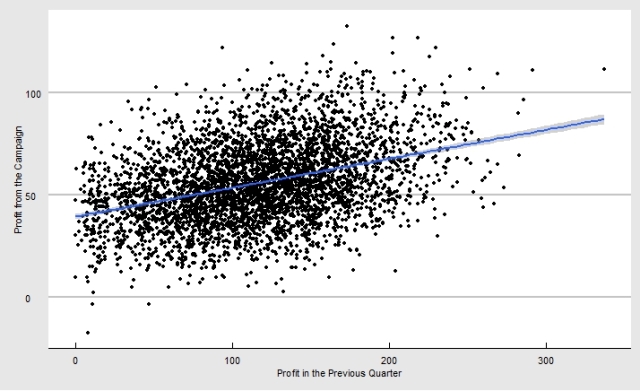
Let’s come back to our case study example and create a regression model to estimate the profitability of every customer for campaign management. In the last part, we have created a simple regression model with a categorical variable i.e. location category for customers (small towns, medium and large cities). This time, around we will examine a continuous variable ‘profit generated by the customers in the previous quarter’ to determine the profit they will generate through campaigns. The following is the scatter plot for these two variables:
Regression Model
There is a definite correlation between the above variables. If we calculate the correlation coefficients or Carl Pearson product moment for them we get a highly significant value as displayed below:
Correlation Coefficient (ρ)= 0.372
The relationship between these two variables is mostly correlation. Profit in the previous quarter is definitely not causing profit from the campaigns. However, both these variables are governed by the same unobserved factors (driving forces) such as customers’ affinity of purchasing from the online store, and their capability to spend. Hence, this correlation is not spurious or coincidental. As an analyst, it is absolutely important to distinguish between correlation, and coincidence through rigorous logic.
Now, let’s create a simple regression model between these two variables
| Regression Model | Estimate | Std. Error | t Value | Pr(>|t|) |
| (Intercept) | 39.78 | 0.683 | 58.25 | <2e-16 |
| Profit in the Previous Quarter | 0.14 | 0.005 | 25.96 | <2e-16 |
| Multiple R-squared: | 0.138 | |||
| Adjusted R-squared: | 0.138 | |||
| F-statistic (P Value) | 2.2E-16 | |||
The following is the linear equation for the above regression model

The model explains about 13.8% (R-square) variation in ‘profit from the campaign’.
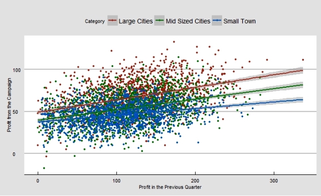
Now, let us extend this model by adding the categorical variable from the last time i.e. ‘category of the location’. Let us first create the same scatter plot with the overlay of this categorical variable.
Regression Model by Category
In theory, you expect the above 3 lines for ‘location category’ to be perfectly parallel to each other. However, in practice, you will rarely find perfectly parallel (or zero interaction) lines. In our case the lines are following the same trend with very little interaction hence we can just add this categorical variable in our above model. The following is the new model after adding ‘location category’:
| Regression Model | Estimate | Std. Error | t Value | Pr(>|t|) |
| (Intercept) | 33.95 | 0.686 | 49.47 | <2e-16 |
| Large Cities | 19.24 | 0.634 | 30.34 | <2e-16 |
| Mid-Sized Cities | 7.29 | 0.626 | 11.64 | <2e-16 |
| Profit in the Previous Quarter | 0.11 | 0.005 | 23 | <2e-16 |
| Multiple R-squared: | 0.296 | |||
| Adjusted R-squared: | 0.295 | |||
| F-statistic (P Value) | 2.20E-16 | |||
Notice, that the adjusted R-square value for this combined model (0.295) is greater than individual continuous (0.138) or categorical (0.2065) variable regression models. This is the process of regression model development where every incremental variable inclusion in the model will improve the R-squared value.
Sign-off Note
Determinism philosophy of science believes that if one has the complete / absolute knowledge of the Universe then one can predict the fate of the Universe with 100% accuracy or 100% R-squared value. However, quantum mechanics has created serious doubts in the deterministic view of the Universe. Mother Nature is an enigma – full of new tricks – this is possibly the greatest source of her eternal beauty.
See you soon with a new article.
Hello Roopam. I just want to thank you for creating this retail case study series. I’ve read every part and am truly impressed with your detailed yet very understandable explanations. Keep them coming!
Thanks Ellen, am glad you are enjoying my blog posts.
I have done statistical modeling but never seen such wonderful/simple explanations. Looking forward to more from you. Congratulations.
Thanks Karra
Very good explanations
Thanks Karan!
Amazing article. Do you have any post on sampling (size etc) strategy and approach for test and control purposes (Bnaking/Credit Cards).
Hi Girish,
Thanks for the kind words. Let me share a piece from a previous article on sampling strategy, hope you will find it useful:
—
A few years ago, I did a daylong workshop on Statistical Inference for a large German shipping & cargo company in Mumbai. At the time of Q&A session the Vice President of operations asked a tricky question, what is a good sample size to achieve good precision? He was looking for a one-size-fit-all answer and I wish it were that simple. The sample size depends on the degree of similarity or homogeneity of the population in question. For example, what do you think is a good sample size to answer the following two questions?
1. What is the salinity of the Pacific Ocean?
2. Is there another planet with intelligent life in the Universe?
In terms of population size, number of drops in the ocean and planets in the Universe is similar. A couple of drops of water are enough to answer the first question since the salinity of oceans is fairly constant. On the other hand, second question is a black swan problem. You may need to visit every single planet to rule our possibility of intelligent form of life.
For credit scorecard development and other classification problems, the accepted rule of thumb for sample size is at least 1000 records of both good and bad loans. There is no reason why you cannot built a scorecard with a smaller sample size (say 500 records). However, the analyst needs to be cautious in doing so because a higher degree of randomness creeps in a small data sample. Additionally, it is also advisable to keep the sample window as short as possible i.e. a financial quarter or two while scorecard development. Further, the sample is divided into two pieces – usually, 70 % for development and remaining for validation sample.
Link to the above article
Thank you. The content of your blog has been very helpfull for me. I’m looking forward to read about a New case study example.
Thanks Roopam
I am following your post from long time. you always make things easier to understand. Thanks
Thanks Muhammad, am glad you are finding the posts on YOU CANalytics helpful.
Hi Roopam, your articles are excellent! Thank you.
btw part 9 and others too are missing of this page.
Best,
Luke