In this article we are going to discuss Bayesian inference and statistics. In order to gain understanding of Bayesian inference we will use the experiment of coin tossing. Hence it is only appropriate to have a quick discussion about the power of…

…Flip of the Coin

To begin with, let me pay my tribute to the master of randomness and the most flippant of them all – the act of tossing a coin.

O’ you epitome for fickleness
     O’ you undisputed lord of chance,
May no game ever begin without
    Your approval and mystical dance.

The Mystical Dance – by Roopam

When I was in high school, I always use to wonder why tossing coins were such an integral part of probability theory. Almost every basic, intermediate or advanced book on probability has more than a few references to coin tosses. The reason, I figured out later, is that tossing a coin is one of the easiest and fastest experiments with random binary outcomes. The following are some of the practical events with random binary outcomes where one is trying to identify –

– Fraudulent transactions
– Customers for cross/up selling
– Malignant cancer cells
– Credit risk of a customer
– Spam emails
– Employees likely for attrition

All these events are in principal similar to tossing coins. The major difference for these events to tosses is that it will take several months to register the outcomes of these events – unlike heads and tails. In the subsequent segments, we’ll discuss Bayesian statistics through coin tosses.

Frequentist and Bayesian Inference

If one has to point out the most controversial issue in modern statistics, it has to be the debate on Frequentist and Bayesian statistics. Frequentist or Fisherian statistics (names after R. A. Fisher) is something that is often employed in most scientific investigation, though there are enough doubts raised about Frequentist logic (read The Signal and The Noise by Nate Silver). Irrespective of the controversies, it is essential for a pragmatic analyst to understand the difference and application of both these approaches.

Frequentist approach is based on setting a testable hypothesis and collecting samples to accept or reject this hypothesis. The Bayesian inference on the other hand modifies its output with each packet of new information. I have discussed Bayesian inference in a previous article about the O. J. Simpson case; you may want to read that article. If you could recall setting a prior probability is one of the key aspects of Bayesian inference. Defining prior probability also makes the analyst think carefully about the context for the problem as this requires a decent understanding of the system. We will get a first-hand experience of this in the example to follow.

Bayesian Inference

Let’s assume that there is a company that makes biased coins i.e. they adjust the weight of the coins in such a way that the one side of the coin is more likely than the other while tossing. For a time being assume that they make just two types of coins. ‘Coin 1’ is 30% likely to give heads (rather than 50% for an unbiased coin) and ‘Coin 2’ is 70% likely to give heads. Now, you have got a coin from this factory and want to know if it is ‘Coin 1’ or ‘Coin 2’. At this point you have inquired about the production system of the company that produces both types of coin in the same quantity. This will help you define you prior probability for the problem that is your coin is equally likely to be either ‘Coin 1’ or ‘Coin 2’ or 50-50 chance.

After assigning prior probability, you have tossed the coin 3 times and got heads in all three trials. The Frequentist approach will ask you to take more samples since one cannot accept or refuse the null hypothesis with this sample size at 95% confidence interval. However, as we will see with Bayesian approach each packet of information or trial will modify the prior probability or your belief for the coin to be ‘Coin 2’.

At this point we know the original priors for the coins i.e.

Additionally we also know the conditional probability i.e. chances of heads for Coin 1 and Coin 2

Now we have performed our first experiment or trial and got heads. This is a new information for us and this will help calculate the posterior probability of coins when heads has happened (recall for our previous article read that article)

If we insert the values to the above formula the chances for Coin1 have gone down

Similarly chances for Coin 2 have gone up

This same experiment is shown in the figure below:

As mentioned in the above figure the posterior probabilities of the first toss i.e. P(Coin 1|Heads) and P(Coin 2|Heads) will become the prior probabilities for the subsequent experiment. In the next two experiments we have further got 2 more heads this will further modify the priors for the fourth experiment as shown below. Each packet of information is improving your belief about the coin as shown below.

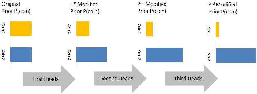
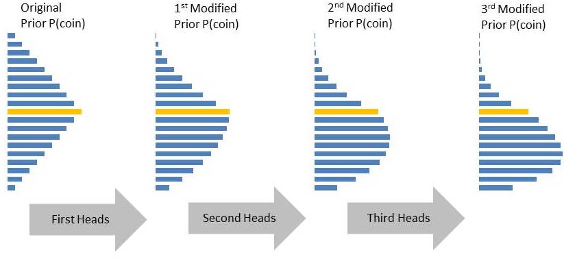
By the end of the 3rd experiment you are almost 93% sure that you have a coin that resembles Coin 2. The above example is a special case since we have considered just two coins. However, for most practical problems you will have factories that produce coins of all different biases (remember toss of coin is a synonym for the more practical problems we have discussed above). In such cases the prior probabilities will be a continuous distribution (a case for triangle distribution as shown below). Notice with the results of each experiment how bulge is shifting toward coins that are more likely to produce heads. Keep in mind the orange bar in the figure below is for the unbiased coin i.e. 50/50 chances for heads and tails.

Sign-off Note

As I am learning more about Bayesian Inference, I must say as an analyst my affinity or bias is leaning towards Bayesian over Frequentist. However, in the same breath I must also point out that setting Bayesian priors and calculation for Bayesian statistics are effort intensive. Additionally, in absence of a proper prior selection Bayesian inference can produce similar or worse results compared to Frequentist approaches. As mentioned Bayesian approaches require better understanding of context and the system of interest. See you soon.